worksheet grid lines

Show or hide gridlines on a worksheet

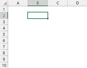
Gridlines are the faint lines that appear between cells on a worksheet.

Worksheet in which gridlines are showing

About gridlines

When working with gridlines, consider the following:

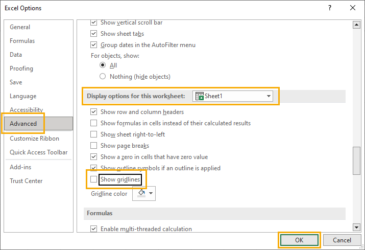
By default, gridlines are displayed in worksheets using a color that is assigned by Excel. If you want, you can change the color of the gridlines for a particular worksheet by clicking Gridline color under Display options for this worksheet ( File tab, Options , Advanced category).

People often confuse borders and gridlines in Excel. Gridlines cannot be customized in the same manner that borders can. If you want to change the width or other attributes of the lines for a border, see Apply or remove cell borders on a worksheet .

Note: You must remove the fill completely. If you change the fill color to white, the gridlines will remain hidden. To keep the fill color and still see lines that serve to separate cells, you can use borders instead of gridlines. For more information, see Apply or remove cell borders on a worksheet .

Gridlines are always applied to the whole worksheet or workbook, and can't be applied to specific cells or ranges. If you want to apply lines selectively around specific cells or ranges of cells, you should use borders instead of, or in addition to, gridlines. For more information, see Apply or remove cell borders on a worksheet .

Hide gridlines on a worksheet

If the design of your workbook requires it, you can hide the gridlines:

Worksheet in which gridlines have been hidden

Select one or more worksheets .

Tip: When multiple worksheets are selected, [Group] appears in the title bar at the top of the worksheet. To cancel a selection of multiple worksheets in a workbook, click any unselected worksheet. If no unselected sheet is visible, right-click the tab of a selected sheet, and then click Ungroup Sheets .

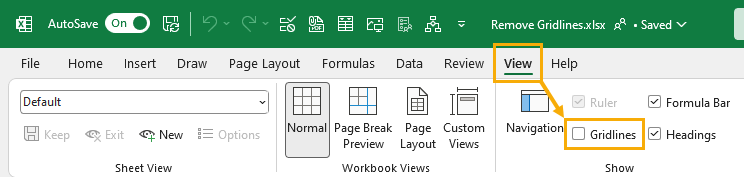
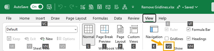
On the View tab, in the Show group, clear the Gridlines check box.

Show gridlines on a worksheet

If the gridlines on your worksheet are hidden, you can follow these steps to show them again.

On the View tab, in the Show group, select the Gridlines check box.

Note: Gridlines do not print by default. For gridlines to appear on the printed page, select the Print check box under Gridlines ( Page Layout tab, Sheet Options group).

Select the worksheet.

Click the Page Layout tab.

To show gridlines: Under Gridlines , select the View check box.

To hide gridlines: Under Gridlines , clear the View check box.

Gridlines are used to distinguish cells on a worksheet. When working with gridlines, consider the following:

By default, gridlines are displayed on worksheets using a color that is assigned by Excel. If you want, you can change the color of the gridlines for a particular worksheet.

People often confuse borders and gridlines in Excel. Gridlines cannot be customized in the same way that borders can.

If you apply a fill color to cells on a worksheet, you won't be able to see or print the cell gridlines for those cells. To see or print the gridlines for these cells, you must remove the fill color. Keep in mind that you must remove the fill entirely. If you simply change the fill color to white, the gridlines will remain hidden. To retain the fill color and still see lines that serve to separate cells, you can use borders instead of gridlines.

Gridlines are always applied to the entire worksheet or workbook and can't be applied to specific cells or ranges. If you want to selectively apply lines around specific cells or ranges of cells, you should use borders instead of, or in addition to, gridlines.

You can either show or hide gridlines on a worksheet in Excel for the web.

On the View tab, in the Show group, select the Gridlines check box to show gridlines, or clear the check box to hide them.

Excel for the web works seamlessly with the Office desktop programs. Try or buy the latest version of Office now.

Show or hide gridlines in Word, PowerPoint, and Excel

Print gridlines in a worksheet

Need more help?

Want more options.

Explore subscription benefits, browse training courses, learn how to secure your device, and more.

Microsoft 365 subscription benefits

Microsoft 365 training

Microsoft security

Accessibility center

Communities help you ask and answer questions, give feedback, and hear from experts with rich knowledge.

Ask the Microsoft Community

Microsoft Tech Community

Windows Insiders

Microsoft 365 Insiders

Was this information helpful?

Thank you for your feedback.

PRO Courses Guides New Tech Help Pro Expert Videos About wikiHow Pro Upgrade Sign In
EDIT Edit this Article
EXPLORE Tech Help Pro About Us Random Article Quizzes Request a New Article Community Dashboard This Or That Game Popular Categories Arts and Entertainment Artwork Books Movies Computers and Electronics Computers Phone Skills Technology Hacks Health Men's Health Mental Health Women's Health Relationships Dating Love Relationship Issues Hobbies and Crafts Crafts Drawing Games Education & Communication Communication Skills Personal Development Studying Personal Care and Style Fashion Hair Care Personal Hygiene Youth Personal Care School Stuff Dating All Categories Arts and Entertainment Finance and Business Home and Garden Relationship Quizzes Cars & Other Vehicles Food and Entertaining Personal Care and Style Sports and Fitness Computers and Electronics Health Pets and Animals Travel Education & Communication Hobbies and Crafts Philosophy and Religion Work World Family Life Holidays and Traditions Relationships Youth
Browse Articles
Learn Something New
Quizzes Hot
This Or That Game
Train Your Brain
Explore More
Support wikiHow
About wikiHow
Log in / Sign up
Computers and Electronics
Spreadsheets
Microsoft Excel

3 Easy Ways Add Grid Lines to Your Excel Spreadsheet

Last Updated: March 11, 2024 Fact Checked

Enabling Gridlines (Windows)

Enabling gridlines (mac), adding cell borders.

This article was co-authored by wikiHow staff writer, Rain Kengly . Rain Kengly is a wikiHow Technology Writer. As a storytelling enthusiast with a penchant for technology, they hope to create long-lasting connections with readers from all around the globe. Rain graduated from San Francisco State University with a BA in Cinema. There are 8 references cited in this article, which can be found at the bottom of the page. This article has been fact-checked, ensuring the accuracy of any cited facts and confirming the authority of its sources. This article has been viewed 127,375 times. Learn more...

Grid lines, which are the faint lines that divide cells on a worksheet, are displayed by default in Microsoft Excel. You can enable or disable them by worksheet, and even choose to see them on printed pages. These are different from cell borders, which you can add to cells and ranges and customize with line styles and colors. Here's how to add grid lines to your Excel spreadsheet on Windows and Mac computers.

Showing Gridlines in Excel for Windows

To display the default gridlines on your Excel worksheet, click View at the top. Find the Show section and check the box for Gridlines . [1] X Trustworthy Source Microsoft Support Technical support and product information from Microsoft. Go to source
To print the gridlines, click Page Layout → Sheet Options → check the box for Print underneath Gridlines . [2] X Trustworthy Source Microsoft Support Technical support and product information from Microsoft. Go to source
For more border customizations, add a cell border to your data instead.

Gridlines can't be customized in the same way borders can. For more customization options with cell borders, see this section .

You should see a list of options, such as Ruler, Gridlines, Formula Bar, etc. [4] X Trustworthy Source Microsoft Support Technical support and product information from Microsoft. Go to source

Click the Page layout tab at the top.
Find the Sheet Options section.
Check the box next to Print underneath Gridlines .

Step 1 Open a worksheet in Microsoft Excel.

If you want to print with the gridlines on, check the box next to Print .

Gridlines appear on all sheets by default, but they may not be bold enough to make your data stand out. If you want to surround certain data with more visible lines, you can add borders to those cells.

Step 2 Select the range of cells you want to add borders to.

To customize the actual line used in the border (such as changing a solid line to a dotted line), select one of the line styles from the Styles area.
To make the border a different color, choose a color from the Color menu.

To remove cell borders, click the arrow next to the Borders icon in the toolbar, and then choose No Border .
Unlike gridlines, cell borders are always shown on printed sheets.

Expert Q&A

↑ https://support.microsoft.com/en-gb/office/show-or-hide-gridlines-on-a-worksheet-3ef5aacb-4539-4ad5-9945-5ed53772dc4d
↑ https://support.microsoft.com/en-gb/office/print-gridlines-in-a-worksheet-fdb32f2a-8a5a-41fe-a5b0-0a734fdfade1
↑ https://support.microsoft.com/en-us/office/create-a-new-workbook-ae99f19b-cecb-4aa0-92c8-7126d6212a83
↑ https://support.microsoft.com/en-us/office/show-or-hide-gridlines-on-a-worksheet-3ef5aacb-4539-4ad5-9945-5ed53772dc4d#OfficeVersion=Windows
↑ https://support.microsoft.com/en-us/office/show-or-hide-gridlines-in-word-powerpoint-or-excel-47b1189c-f867-479e-a208-34ee54055f6f
↑ https://support.microsoft.com/en-gb/office/show-or-hide-gridlines-on-a-worksheet-3ef5aacb-4539-4ad5-9945-5ed53772dc4d#OfficeVersion=macOS
↑ https://support.microsoft.com/en-us/office/apply-or-remove-cell-borders-on-a-worksheet-dc8a310b-92e3-46a7-9f17-2ab745810f4a

About This Article

1. Click the File menu and select Options . 2. Click Advanced . 3. Select the sheet from the "Display options for this worksheet" menu. 4. Check the box next to "Show gridlines." 5. Click OK . Did this summary help you? Yes No

Send fan mail to authors

Is this article up to date?

Featured Articles

Watch Articles

Terms of Use
Privacy Policy
Do Not Sell or Share My Info
Not Selling Info

wikiHow Tech Help Pro:

Level up your tech skills and stay ahead of the curve

Ablebits blog
Excel formatting

How to show and hide gridlines in Excel

In the previous blog post we successfully solved the problem of Excel not printing gridlines . Today I'd like to dwell on another issue related to Excel grid lines. In this article you'll learn how to show gridlines in an entire worksheet or in certain cells only, and how to hide lines by changing cells background or borders' color.

When you open an Excel document, you can see the horizontal and vertical faint lines that divide the worksheet into cells. These lines are called gridlines. It is very convenient to show gridlines in Excel spreadsheets as the key idea of the application is to organize the data in rows and columns. And you don't need to draw cell borders to make your data-table more readable.

Sample worksheet with and without gridlines

Whether you decide to show gridlines in your worksheet or hide them, go ahead and find below different ways to fulfil these tasks in Excel 2016, 2013 and 2010.

Show gridlines in Excel

Suppose you want to see gridlines in the entire worksheet or workbook, but they are just turned off. In this case you need to check one of the following options in the Excel 2016 - 2010 Ribbon.

Start with opening the worksheet where cell lines are invisible.

Note: If you'd like to make Excel show gridlines in two or more sheets, hold down the Ctrl key and click the necessary sheet tabs at the bottom of the Excel window. Now any changes will be applied to every selected worksheet.

Select the Gridlines checkbox on the VIEW tab to show gridlines in Excel

Whichever option you choose gridlines will instantly appear in all the selected worksheets.

Note: If you want to hide gridlines in the entire spreadsheet, just uncheck the Gridlines or View options.

Show / hide gridlines in Excel by changing the fill color

One more way to display / remove gridlines in your spreadsheet is to use the Fill Color feature. Excel will hide gridlines if the background is white. If the cells have no fill, gridlines will be visible. You can apply this method for an entire worksheet as well as for a specific range. Let's see how it works.

Tip: The easiest way to highlight the whole worksheet is to click on the Select All button in the top-left corner of the sheet.

Click the Select All button in the top-left corner to highlight the entire spreadsheet

Go to the Font group on the HOME tab and open the Fill Color drop-down list.

Note: If you want to show lines in Excel, pick the No Fill option.

Choose the white color from the Fill Color drop-down list to hide gridlines

Make Excel hide gridlines only in specific cells

In case you want Excel to hide gridlines only in a certain block of cells, you can use the white cells background or apply white borders. Since you already know how to change the background color , let me show you how to remove gridlines by coloring the borders.

Select the block of cells where you want to remove gridlines

Note: You can also use the Ctrl + 1 keyboard shortcut to display the Format Cells dialog.

Make sure that you are on the Border tab in the Format Cells window.

Choose the white color and press Outline and Inside to hide gridlines in the block of cells

Note: To bring gridlines back to the block of cells, choose None under Presets in the Format Cells dialog window.

Remove gridlines by changing their color

You see there are different ways to show and hide gridlines in Excel. Just choose the one that will work best for you. If you know any other methods of showing and removing cell lines, you are welcome to share them with me and other users! :)

55 comments

That was such an sharp and clear tutorial: thank you so much for doing it :)

Thank you for such a clear useful tutorial!

thanks for the given support to resolve the my task. very useful those guideline for everyone's.

I had gridlines disappear from cells after I removed those cell's borders. It turned out that my Conditional Formatting for those cells was the problem - I had told the cells to turn white instead of having them change to no colour.

How to show gridlines when cells are filled woth colour? They always disappear when i fill with colour

I want to retain certain data based on their column number and delete the rest

I want to sellect certain number from the column and delete the rest. Note The data are large

I only want to copy the number inside a certain cell to the other cell having different border format. The problem is, the border were also copied. How am I suppose to do?

Hello Manny! If you use the key shortcuts CRTL+C / CRTL+V or the Copy / Paste options from the context menu, you copy not only formulas or values, but the format of the cells as well. If you want to copy just values, please use the Paste Special option from the context menu or the CRTL+ALT+V key shortcut. In the dialog window opened please choose what exactly you want to insert into a cell.

Thank you! Very helpful!

I have Excel 2000 and came across this page! I found a solution to remove grid lines by selecting "View" then "Toolbars" and selecting "Forms" from the drop down menu. Make sure "Forms" is checked on. You can then select on this toolbar "Toggle Grid" and that did it for me!

I had to leave this page. The info may or may not be helpful, but the giant, moving, animated bullshit running across the bottom was way too distracting. I will not be back to this page.

Thank you, very helpful!

Thanks for the tip. it was helpful.

I want to make the text of a cell disappear if the adjacent cell is blank. Or the reverse: when text is entered into a cell, a specified number appears in the adjacent cell.

Excellent, thank you!

None of these suggestions worked for me, I ended up figuring it out myself ... after wayyyy too long: Go to the Home tab Go to the Font section Select the little square table icon Select All Borders Gridlines have returned! I have maybe three strands of hair left after pulling out the rest. Hope this helps someone.

Thanks Fluke! Came here years after, and nothing worked, but that worked. It's not perfect, but I'll take it.

Thank you!!!!! Seriously. SOOOOO MUCH!!! :)

Almost... the lines are back, but they aren't the same color as the default; now they're darker. There should be a button that says, "don't EVER mess with the grids." I can't be the only one.

thanks a lot . very useful information

gridlines go off when setting a bg color how do you fix this ?

Awesome Thanks

how to turn on a grid lines in excel?

Thanks a lot! I work well!

Thanks, no response expected!!!

Thank you this was very helpful, I was trying to get the lines back in certain cells only and this really helped me figure it out.

Sometimes you find a set of three cells (arranged vertically) plus one more to the right of the middle one of the three, with no gridlines showing between them. In this case it seems (sometimes) that that middle one has been formatted unexpectedly. To cure, go to Format Cells, select the Fill tab, and click on No Colour (because even if you can't really see it, it turns out that the White button has been selected. This cured a puzzle for us!

This is the answer I've been searching for. Thank you!

This is what I use because I want colors but still wanted the faint gridline to organize the data.

My solution: Highlight the area you want the gridlines (likely the area you colored and lost them) - Right click - format cells - select the normal border size on the bottom left of the style box - under the color option select "Tan, Background 2" (this is a pre-set option third over right on the top selection - next ensure you select the type of border you want (this is the sample box that says "none, outline, inside, etc.) - finally click okay. You should now have a faint grid border that blends with the original grid marks un-noticingly (yes I made that word up :)

You can then use the same steps to add a black border around your new grid like border to better present your colored grid lined chart. :)

Thank you!!! I couldn't find this anywhere.

thank you!!!!

The gridlines only show for the information entered. Meaning, if only two days have been entered so far, gridlines only show up for those two days. I need the whole page to print out in gridlines. Those future gridline days will eventually be filled in.

Hello, I have a problem. When I write two numbers next to each other, the line between them disappears. What should I do? Thanks.

I am steel in problem with office 2013 excel because of gridline. All is checked and nothing

Yes, but is there any way to have both background color (fill) AND gridlines?

I followed all the suggestions on the Web to show gridlines in Excel 2013 to no avail. I have no idea why it suddenly stopped displaying them. Please help.

Just go to view and check the gridlines box.

Allens comment solved my problem, background set to "no fill"

Thank Mark I resolved with your Tips

who r u i dont no but thanks to u god bless u my dear

One reason that grid lines are not showing is that background has been set to white. Select whole sheet, click TLH corner. In Home set background to "no fill".

THANK YOU. I could not work without the lines and it bugged me really badly to see it blank. The second tip helped me.

To fix what you describe, go to the 'Home' tab. On the right hand side of the toolbar, you will see 'Clear'. Click on clear and then select 'Clear Formats'.

That should fix your problem.

I have a spreadsheet I received from someone else. When I look at it on the screen, it looks fine. When it prints (legal/landscape) it is only printing the gridlines on the left half of the paper. I have tried adding borders to the entire document, selecting all and showing/printing gridlines, etc. Nothing seems to work.

Thank you! Saved my morning. My boss isn't here and I didn't want to have to ask him how to do this. So yeah, thanks :D

I attempted to get the gridlines back after removing cell borders and by selecting the area and then presets of 'none' I still cannot get the gridlines back. Any ideas in using Excel 2010?

same problem here

Please change the color type to automatic, choose none and press ok

i am having same problem as Ilka. Please explain step by step. where is the colour type which i have to set as automatic??

7 Ways to Add or Remove Gridlines in Microsoft Excel

This post is going to show you all the different methods you can use to add or remove the gridlines in your Excel workbooks.

Excel has gridlines in each sheet or your workbook. These are the light gray lines that outline each cell in the sheet.

Gridlines can help you distinguish between the rows, columns, and any data they contain. But maybe you don’t want to see the gridlines in your final report or dashboard. In this case, you will want to hide these gridlines.

Removing the gridlines is very easy and it can be done in many ways.

Download a copy of the example workbook used in this post and follow along to discover all the ways you can show or hide the gridlines in your Excel workbooks.

Add or Remove Gridlines from the View Tab

Removing the gridlines is such a common task that it has been included as a command in the Excel ribbon View tab.

This is the most straightforward method for toggling on or off the gridlines.

Follow these steps to toggle on or off the gridlines from the View tab.

Go to the View tab.
Click on the Gridlines option in the Show section.

This will remove the Gridlines from the active sheet when you uncheck the Gridlines option.

Add or Remove Gridlines from the Excel Options Menu

The Excel Options menu is where you will find a ton of useful app and workbook settings to enhance your Excel experience, and you can also find the gridline settings here.

Follow these steps to add or remove the gridlines from the Excel Options menu.

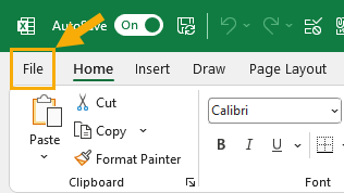
Go to the File tab.

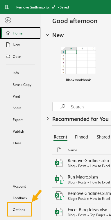
Select Options in the lower left of the backstage screen.

This will open the Excel Options menu.

Go to the Advanced section of the Excel Options menu.
Scroll down to the Display options for this worksheet section and select the sheet in the dropdown from which you want remove the gridlines.
Press the Show gridlines option. Uncheck this to remove the gridlines from the sheet.
Press the OK button to close the Excel Options menu.

This will remove the gridlines from your sheet!

Add or Remove Gridlines with a Keyboard Shortcut

There is no dedicated keyboard shortcut to add or remove the gridlines in Excel, but you can use the Alt hotkeys.

When you press the Alt key, this will activate the hotkeys and the Excel ribbon will display what keys you need to press in order to navigate the ribbon commands.

Press the Alt , W , V , G sequence on your keyboard to toggle on or off the gridlines with a keyboard shortcut.

Add or Remove Gridlines from the Quick Access Toolbar

One way to make removing the gridline very easy is to add this command to your Quick Access Toolbar.

This way it is always accessible with one click.

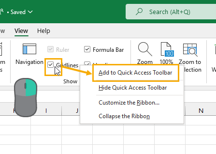
Follow these steps to add the gridline command to your quick access toolbar.

Right-click on the Gridline option.
Select the Add to Quick Access Toolbar option from the menu.

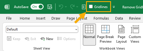
Now the command will be available in your Quick Access Toolbar!

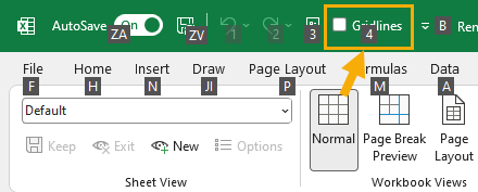
💡 Tip : The Alt hotkeys are an easy way to use the commands in your Quick Access Toolbar! In this example, the Gridlines command is the 4th item in the QAT so you can press Alt + 4 to access it.

Add or Remove Gridlines when Printing

If you want to print your Excel reports, the gridlines don’t appear in the printed results by default.

However, you may want the gridlines to appear and it is possible to have them show in the printouts.

Follow these steps to add or remove the gridlines to your Excel printouts.

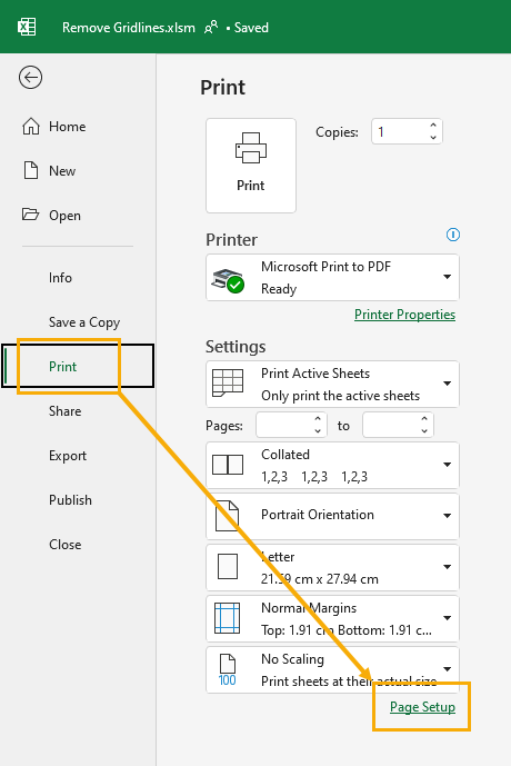
Go to the Print options.
Click on the Page Setup link at the bottom of the printing options.

This will open the Page Setup menu.

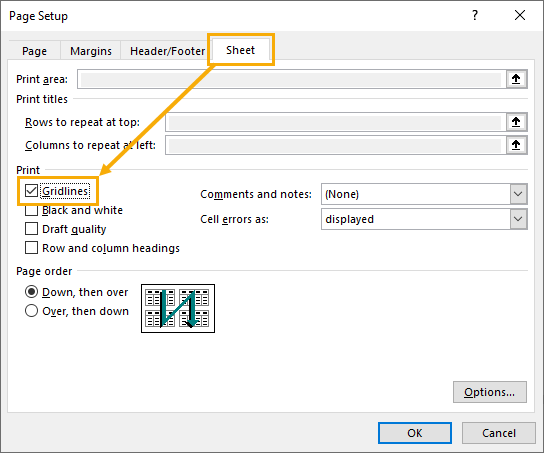
Go to the Sheet tab in the Page Setup menu.
Check the Gridlines options under the Print section.
Press the OK button.

Now your printouts will show the gridlines!

Add or Remove Gridlines from All Sheets with VBA

The methods you have seen so far for removing gridlines have one major issue. If you want to remove gridlines from all the sheets in your workbook, you will have to change the gridline setting for each sheet individually.

This can be a very tedious process when you have a lot of sheets in your workbook.

You can use a VBA script to automate this process and remove the gridlines from all the sheets at once.

Go to the Developer tab and click on the Visual Basic command to open the visual basic editor.

If you don’t find this tab in your ribbon, you can easily add the Developer tab to your ribbon . You can also press Alt + F11 on your keyboard to open the editor.

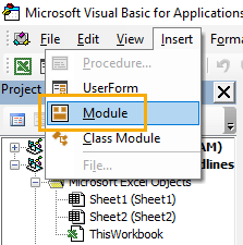
Go to the Insert menu and select the Module option to create a new module. This is where you can add the VBA code that will remove the gridlines in all the sheets of the workbook.

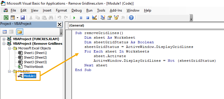
Select the new module and then paste in the above code.

This code will loop through all the sheets and toggle on or off the gridlines depending on the gridline status of the sheet in view when you run the macro .

This is a quick way to toggle gridlines for all the sheets!

Add or Remove Gridlines from All Sheets with Office Scripts

There is another option for automating the removal of the gridlines from all your sheets.

If you are using Excel online with a business plan, then you will have access to Office Scripts. This is a JavaScript language that can be run for Excel on the web!

You can create an Office Script to toggle on or off the gridlines from your entire workbook.

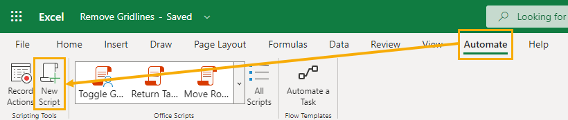
Go to the Automate tab in Excel online and select the New Script command.

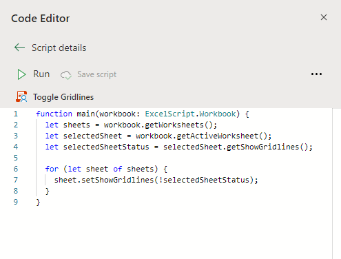
This will open the Office Script editor and you can copy and paste the above code into the editor.

This code will loop through all the sheets in the workbook and toggle on or off the gridlines based on the gridline status of the current sheet.

Press the Run button in the editor to run this code and easily switch between showing or hiding the gridlines while using Excel on the web.

Conclusions

By default, light gray lines separate each cell in your workbook, but you can remove these lines for a much cleaner look to your Excel reports and dashboards.

The gridline settings can be found in either the View tab or the Excel Options menu and these will toggle on or off the gridlines on a per sheet basis.

When printing your Excel reports, it is also possible to include the gridlines if needed.

You can also use VBA or Office Scripts to automate the process of removing gridlines in all your sheets. This is essential when you have a workbook with many sheets.

Do you like the default gridlines or do you prefer to remove than from your workbooks? Do you know any other ways to get this done? Let me know in the comments section below!

About the Author

John MacDougall

Subscribe for awesome Microsoft Excel videos 😃

I’m John , and my goal is to help you Excel!

You’ll find a ton of awesome tips , tricks , tutorials , and templates here to help you save time and effort in your work.

Pivot Table Tips and Tricks You Need to Know
Everything You Need to Know About Excel Tables
The Complete Guide to Power Query
Introduction To Power Query M Code
The Complete List of Keyboard Shortcuts in Microsoft Excel
The Complete List of VBA Keyboard Shortcuts in Microsoft Excel

What is an Absolute Reference in Excel?

May 10, 2024

Wondering what is an absolute reference in Excel? Read this essential Excel...

What Does $ Mean in Excel?

May 9, 2024

What does $ mean in Excel? Read on to learn everything you need to know about...

7 Way to Unprotect a Sheet in Microsoft Excel

May 8, 2024

Want to learn how to unprotect Excel sheets? Read this Microsoft Excel...

Get the Latest Microsoft Excel Tips

Working with Gridlines in Excel: How to Add, Remove, Change, and Print Gridlines

Gridlines in Excel are those faint gray lines that you see around the cells in the worksheet. These gridlines make it easier to differentiate between the cells and read the data.

Now don’t confuse gridlines with borders. Gridlines are visible on the entire worksheet while borders can be applied to the entire worksheet or to a selected region in the worksheet.

You can change border settings such as color, width, style, etc., but in the case of gridlines, you get limited options to change the look of the gridlines.

This Tutorial Covers:

Working with Gridlines in Excel

In this tutorial, you’ll learn:

How to remove gridlines from the entire worksheet.
How to show gridlines in a specific area in the worksheet.
How to change the color of the gridlines.
How to print the gridlines.

How to Remove Gridlines in Excel Worksheets

By default, gridlines are always visible in an Excel worksheet. Here are the steps to remove these gridlines from the worksheet:

Go to the Page Layout tab.
In the Sheet Options group, within Gridlines, uncheck the View checkbox.

This would remove the gridlines from the Excel worksheet.

Here are some things to keep in mind when tinkering with the gridlines:

You can also use the keyboard shortcut – ALT + WVG (hold the ALT key and enter W V G). This shortcut would remove the gridlines if it is visible, else it will make it visible.
Removing the gridlines would remove it from the entire worksheet. This setting is specific to each worksheet. If you remove the gridlines from one worksheet, it would still be visible on all the other worksheets.
You can also remove the gridlines by applying a background fill to the cells in the worksheet. If the gridlines are visible, and you apply a fill color in a specific area, you would notice that the gridlines disappear and the fill color takes over. Hence, if you apply the fill color to the entire worksheet, the gridlines wouldn’t be visible. ( Note that you need to remove the fill color to make the gridlines visible ).
If you want to remove the gridlines from all the worksheets at one go, select the worksheets by holding the Control Key and selecting the tabs (this would group sheets together). You would notice that the workbook is in the Group Mode (see the top of the workbook where the name is displayed). Now change the gridlines view setting and it will be applied to all the worksheets. Make sure to Ungroup the sheets (right-click on the tab and select ungroup) else all the changes you do in the current sheet would also be reflected in all the worksheets.
By default, gridlines are not printed.

How to Show Gridlines in a Specific Area in the Worksheet

In Excel, you can either have the gridline visible in the entire worksheet or hide it completely. There is no way to show this in a specific area.

However, you can use borders to give a gridline effect in a specific area in the worksheet. Borders come with a lot of options and you can make it look exactly like gridlines (by selecting a light gray color).

Note: Unlike gridlines, borders are always printed.

Changing the Color of the Gridlines in Excel

You can choose to have a different gridline color in your Excel worksheets.

To set the default color:

Go to File –> Options.
Make sure to Ungroup the sheets (right click on the tab and select ungroup) else all the changes you do in the current sheet would also be reflected in all the worksheets.
It doesn’t change the default color. The next time you insert a new worksheet or open a new workbook, it would still show the light gray color gridlines.

Printing the Gridlines in Excel

By default, gridlines in Excel are not printed. If you want to print the gridlines as well, make the following change:

Go to Page Layout tab.
In the Sheet Options group, within Gridlines, check the Print checkbox.

While the gridlines aren’t printed by default, borders are always printed.

You May Also Like the Following Tutorials:

How to Insert Page Numbers in Excel Worksheets.
How to Insert Watermark in Excel Worksheets.
How to Insert and Use a Checkbox in Excel.
How to Insert Bullets in Excel
How to Remove Dotted Lines in Excel
How to Split a Cell Diagonally in Excel (Insert Diagonal Line)

FREE EXCEL BOOK

Get 51 Excel Tips Ebook to skyrocket your productivity and get work done faster

How to Remove or Add Gridlines in Excel

Add and remove gridlines to make your spreadsheets pop

University at Buffalo

What Are Gridlines and How Do They Work?

Change the Gridline Colors for the Whole Worksheet

Change the Fill Color to Remove Excel Gridlines

Hide Gridlines for Particular Columns and Rows
Turn Gridlines On and Off for the Whole Worksheet

When a Microsoft Excel Spreadsheet is created, have you ever wondered what the tiny vertical and horizontal lines are called? They're called gridlines, and these lines make up tables and cells. They form an integral part of Excel’s basic functions by letting you organize your data into columns and rows. Gridlines also save you from having to create cell borders to make sure your data is easy to read. That's why it's good to know how to add or remove Excel gridlines.

Most Excel spreadsheets come with gridlines visible as the default setting. However, you may receive a spreadsheet from a co-worker or friend where the gridlines are not visible. You may also decide your data might look better without the gridlines being seen by other users. Either way, adding or removing gridlines is straightforward and doesn't take much time to do.

Several different methods will allow you to show or hide gridlines in Excel 2019, Microsoft 365 , and Excel 2016. These include changing the color of the gridlines themselves, altering the fill color of the worksheet, hiding the gridlines in specific tables and cells, and showing or hiding the gridlines for the entire worksheet.

Change the Color of Excel Gridlines for the Whole Worksheet

Whether you need your gridlines to stand out more or you want to remove them from view, you can change the default gridline color with ease.

The default color of gridlines in worksheets is a light gray, but you can change the color to white to remove your gridlines. If you want to make them visible again, just go back to the menu and select a new color.

In the worksheet for which you want to change the gridline colors, go to File > Options .

Select Advanced .

Under the Display options for this worksheet group, use the Gridline color drop-down menu to select the desired color.

After selecting the desired color, Excel 2016 users must select OK to confirm their choice.

Click Select All (the triangle in the top left corner of the worksheet) or press Ctrl+A .

From the Home tab, select Fill color , then choose the white option. All gridlines will be hidden from view.

In Microsoft Excel, the Fill color menu is represented by a paint bucket icon.

If you want to return the gridlines, select the entire worksheet and select No Fill from the Fill Color menu to remove the fill and make the gridlines visible again.

How to Hide Gridlines for Particular Columns and Rows

There may be times when you only want to have a certain section of gridlines removed to provide visual emphasis for those viewing it.

Choose the group of cells where you want to remove the gridlines.

Right-click the highlighted cells and select Format Cells . You can also press Ctrl+1 to get to the menu.

In the Format Cells dialog box, select the Border tab.

Select white from the color drop-down menu, then select Outside and Inside in the Presets group.

Select OK to confirm your selections.

How to Turn Gridlines On and Off for the Whole Worksheet

Occasionally, you might get a spreadsheet from a friend or colleague that's had the gridlines removed or made invisible. There are two options to quickly and easily restore gridlines for the entire spreadsheet.

Open the spreadsheet with the removed gridlines.

If you need to select more than one worksheet, hold Ctrl select the relevant sheets at the bottom of the workbook.

Select the View tab, then select the Gridline box to restore all gridlines.

Alternatively, you can select Page Layout , and then, under the Gridlines settings, select View .

Get the Latest Tech News Delivered Every Day

The 12 Best Tips for Using Excel for Android in 2024
How to Make a Schedule in Excel
How to Highlight and Find Duplicates in Google Sheets
How to Remove Duplicates in Excel
The 5 Best Spreadsheet Apps for Android in 2024
How to Link or Insert Excel Files to Word Documents
How to Create a Column Chart in Excel
What Is a Spreadsheet Cell?
How to Make and Format a Line Graph in Excel
How to Merge and Unmerge Cells in Excel
Understand the Basic Excel Screen Elements
The 23 Best Excel Shortcuts
How to Highlight in Excel
How to Create a Scatter Plot in Excel
How to Create a Database in Excel
How to Hide and Unhide Columns and Rows in Excel

How to Show or Hide Gridlines in Excel

Show or Hide Gridlines in Excel Worksheets (+ Shortcuts)

by Avantix Learning Team | Updated October 15, 2023

Applies to: Microsoft ® Excel ® 2013, 2016, 2019, 2021 and 365 (Windows)

You can remove or hide gridlines in Excel worksheets to simplify worksheet design. By default, gridlines are displayed but do not print. Gridlines are applied to entire worksheets or workbooks, not to specific cells. If you show or hide gridlines on one worksheet, it doesn't affect other sheets in the same workbook.

Borders and gridlines are two different things. Borders print by default and gridlines do not. You can't change the thickness or some other attributes of gridlines but you can change the thickness and style of borders and apply them to specific cells.

Gridlines may disappear for specific cells if you apply a fill color to cells. In this case, if you want to view or print gridlines, you need to remove the fill color from the selected cells. To remove fill color, select the cells with the fill color you want to remove, click the arrow next to Fill Color on the Home tab in the Ribbon (in the Font group) and select No Fill (not white).

In this article, we'll review how to:

Hide or remove gridlines

Show gridlines, show or hide gridlines using a keyboard shortcut, change the color of gridlines.

Recommended article: How to Merge Cells in Excel (4 Ways)

Do you want to learn more about Excel? Check out our online (virtual classroom) or in-person Excel courses >

To hide or remove gridlines:

Select the worksheet with the gridlines you want to remove by clicking the sheet tab at the bottom of the Excel workbook. If you want to remove gridlines on multiple sheets, click the first sheet tab and Shift-click the last sheet tab. If you Ctrl-click sheet tabs, you can select non-contiguous sheets.
Click the View tab in the Ribbon.
Uncheck or deselect Gridlines in the Show group.
If you have selected multiple sheets, click any unselected worksheet to exit the grouped state. If no unselected sheet is visible, right-click the tab of a selected sheet and then select Ungroup Sheets from the drop-down menu.

Show gridlines appears in the Show group in the View tab in the Ribbon:

Show group in the View tab in the Ribbon in Excel with Gridlines checkbox.

To show gridlines:

Select the worksheet with the gridlines you want to show by clicking the sheet tab at the bottom of the Excel workbook. If you want to show gridlines on multiple sheets, click the first sheet tab and Shift-click the last sheet tab. If you Ctrl-click sheet tabs, you can select non-contiguous sheets.
Check or select Gridlines in the Show group. A check mark should appear.

To show or hide gridlines using a keyboard shortcut:

Select one or more worksheets.
Press Alt > W > V > G (press Alt then W then V then G). This will show gridlines if they are hidden or hide gridlines if they are showing. Don't forget to ungroup the sheets if you have selected multiple worksheets.

By default, gridlines are displayed in worksheets using a default color (automatic).

To change the color of gridlines:

Click the File tab in the Ribbon.
Click Options. A dialog box appears.
Click Advanced in the categories on the left.
In the Display options for the worksheet section, ensure Gridlines is checked.
Click Gridline color. A drop-down menu appears.
Select the color you want.
Click OK. The color of gridlines will change for the selected worksheets.

The Excel Options dialog box appears as follows with gridline color options:

Excel Options dialog box with gridline color options.

If a user has made gridlines white, other users will typically not recognize that gridline colors have been changed so white is not a good choice.

Subscribe to get more articles like this one

Did you find this article helpful? If you would like to receive new articles, JOIN our email list.

More resources

How to Remove Duplicates in Excel (3 Easy Ways)

How to Lock Cells in Excel (Protect Formulas and Data)

How to Combine First and Last Name in Excel (5 Ways)

How to Insert Multiple Rows in Excel (4 Fast Ways with Shortcuts)

How to Replace Blank Cells in Excel with Zeros (0), Dashes (-) or Other Values

Related courses

Microsoft Excel: Intermediate / Advanced

Microsoft Excel: Data Analysis with Functions, Dashboards and What-If Analysis Tools

Microsoft Excel: Introduction to Power Query to Get and Transform Data

Microsoft Excel: New and Essential Features and Functions in Excel 365

Microsoft Excel: Introduction to Visual Basic for Applications (VBA)

VIEW MORE COURSES >

Our instructor-led courses are delivered in virtual classroom format or at our downtown Toronto location at 18 King Street East, Suite 1400, Toronto, Ontario, Canada (some in-person classroom courses may also be delivered at an alternate downtown Toronto location). Contact us at [email protected] if you'd like to arrange custom instructor-led virtual classroom or onsite training on a date that's convenient for you.

What is Power Query in Excel?

Power Query in Excel is a powerful data transformation tool that allows you to import data from many different sources and then extract, clean, and transform the data. You will then be able to load the data into Excel or Power BI and perform further data analysis. With Power Query (also known as Get & Transform), you can set up a query once and then refresh it when new data is added. Power Query can import and clean millions of rows of data.

How to Stop or Control Green Error Checking Markers in Excel

In Microsoft Excel, errors are flagged with small green marker or triangle in the upper left corner of the cell. However, these indicators display when there may be an error but is, in fact, not an error.

Excel Shortcuts to Zoom In and Out in Your Worksheets (4 Shortcuts)

There are several mouse and keyboard shortcuts you can use to zoom in and out in Excel worksheets. Some of these shortcuts are built-in and others can be created by customizing Excel Options.

Our Courses

Avantix Learning courses are offered online in virtual classroom format or as in-person classroom training. Our hands-on, instructor-led courses are available both as public scheduled courses or on demand as a custom training solution.

All Avantix Learning courses include a comprehensive course manual including tips, tricks and shortcuts as well as sample and exercise files.

VIEW COURSES >

Privacy Overview

Pin it on pinterest.

Print Friendly

Edit Gridlines in Excel (Add, Remove, Change, and Print)

In this article, I will try to give a complete overview of how to edit gridlines in Excel. This article will comprise the procedures for adding, removing, changing, and printing gridlines in Excel worksheets and charts.

An Excel gridline is the faint gray edge around each cell in the worksheet. In addition to making it easier to read the data, these gridlines help to distinguish between the cells. Unlike borders, where you can change color, width, style, etc., gridlines offer limited options for changing their appearance. Let’s learn in detail in the following sections.

Download Practice Workbook

You can download the practice workbook from here.

Removing Gridlines in Excel Worksheets

In order to remove the gridlines in Excel worksheets, go to the View tab and uncheck the Gridlines option.

Showing Gridlines in Specific Area in Worksheet

If you want to have gridlines in a specific area of a worksheet, select that specific area first.
Then, go to the Home tab and select All Borders from the Borders option.

After that, go to the View tab and uncheck the Gridlines .
Thus, we will have gridlines only in a specific area.

Changing Color of Gridlines in Excel

To change the color of gridlines in Excel, select the entire worksheet just by clicking the small triangle at the top-left corner of the worksheet.
Then, go to the File tab.

Next, go to Options .

Go to the Advanced tab from the Excel Options wizard.
Pick a color from the Gridline Color option which is under the Display options for this worksheet group.

Thus, the color of the gridlines will get changed.

Printing Gridlines in Excel

Normally, the gridlines do not get printed.
In order to print the gridlines, go to the page Layout tab and check the Print box under the Gridlines option.

Controlling Chart Gridlines in Excel

Removing chart gridlines.

Select the chart first. The Chart Elements option will appear in the right-top corner.
Uncheck the Gridlines box from the Chart Elements option.

Showing Single or Multiple Gridlines in Excel Chart

In order to have single-type gridlines, select the chart first.
Then go to the right-top corner and click on the Chart Elements option.
Now go to the Gridlines option and pick any one type of gridline (i.e. Primary Minor Horizontal ) from the available ones.

Inserting Single Pattern Chart Gridlines

To have multiple-type gridlines, select as many types of gridlines as you want from the Gridlines option and all of them will be applied to the chart.

Things to Remember

The change in gridline color is only applicable to the selected sheet. The rest of the sheets will have the default color of gridlines.
The editing of the gridlines does not affect the cell formatting.
The gridlines are different from the borders in Excel.

In this article, I have tried to give a complete overview of how to edit gridlines in Excel. This includes how to show/remove, change color, and print gridlines of sheets and some modifications of chart gridlines. I hope this article will be helpful for you. For any further questions, please comment below. You can also visit our site for more Excel-related articles.

Frequently Asked Questions

1. How do I change the spacing between gridlines in Excel?

In order to change the spacing between gridlines in Excel, click on the small triangle at the top-left corner of the worksheet to select the entire sheet. Then, put the cursor on the worksheet area and right-click on the mouse. From the available option, pick the Row Height… option and input your desired spacing between gridlines.

2. Do the gridlines get printed while printing?

By default, the gridlines do not get printed while printing. To print the gridlines, go to the page Layout tab and check the Print box under the Gridlines option.

3. Is it possible to apply gridlines to a certain area?

No, we can not apply gridlines to a certain area in Excel. But we can use the All Borders option from Border Styles to the selected area and then remove the gridlines. This will show borders to only that selected region which can be considered as gridlines for that particular area.

Edit Gridlines in Excel: Knowledge Hub

Change Gridlines to Dash
Make Grid Lines Bold in Excel
Make Gridlines Darker in Excel

<< Go Back to Gridlines | Learn Excel

What is ExcelDemy?

Tags: Excel Gridlines

Naimul Hasan Arif, a BUET graduate in Naval Architecture and Marine Engineering, has been contributing to the ExcelDemy project for nearly two years. Currently serving as an Excel and VBA Content Developer, Arif has written more than 120 articles and has also provided user support through comments His expertise lies in Microsoft Office Suite, VBA and he thrives on learning new aspects of data analysis. Arif's dedication to the ExcelDemy project is reflected in his consistent contributions and... Read Full Bio

How to Add Gridlines in Excel

Written by: Bill Whitman

Last updated: May 20, 2023

Adding gridlines to your Excel worksheet can make it easier to read and understand the data in your table. Gridlines serve as visual aids, helping to differentiate between cells and rows. However, some users may find it difficult to locate and turn on this feature. In this tutorial, we’ll provide a step-by-step guide on how to add gridlines to your Excel sheet.

Step 1: Open the Worksheet

The first step to adding gridlines to your Excel worksheet is to open the worksheet you want to apply the gridlines to.

Step 2: Select the Cells

Select the cells for which you want to apply the gridlines. You can select a single cell, multiple cells, or the entire worksheet.

Step 3: Navigate to the ‘View’ Tab

Navigate to the ‘View’ tab on the ribbon at the top of your screen. This tab contains all of the features related to how your worksheet is displayed.

Step 4: Turn Gridlines on

In the ‘Show’ section of the ‘View’ tab, you will see an option labeled ‘Gridlines.’ Click on this option to turn on gridlines for your selected cells.

If your worksheet already had gridlines, then you won’t see this option enabled in the view tab. But, if it was turned off, then perform this step to turn it back on.

Step 5: Adjust Gridline Color and Style (Optional)

By default, Excel’s gridlines are displayed in a light gray color. If you want to change the color and style of your gridlines, follow these steps:

Select the cells for which you want to modify the gridlines.
Navigate to the ‘Home’ tab on the ribbon.
Click on the drop-down menu next to the ‘Borders’ button.
Select ‘More Borders’ to open the ‘Format Cells’ dialog box.
Choose your preferred gridline color and style from the options available.

Step 6: Save Your Changes

Finally, save your changes by clicking on ‘Save’ or ‘Save As’ in the top left corner of your screen.

Keep in mind that gridlines are only visible on the worksheet, and not on printed or shared copies of the file. Utilize Borders to create a permanent visual aid for your cells, rows, and columns.

Why Do You Need Gridlines in Excel?

Gridlines can be used in making well-organized tables on your spreadsheet. They make a clear separation of rows and columns making it easy to read and understand the data within. They can also save you time when double-checking data entries as single entries became distinct units.

Additionally, Gridlines can be enabled for printing too. This simplifies the printed document further, making it easier to follow the data.

What Are Some Alternatives to Gridlines in Excel?

There are two alternatives to gridlines in Excel, i.e. borders and shading. They are highly customizable and can also be quite helpful and more visually impressive than gridlines.

The Border alternative to gridlines uses lines that highlight particular ranges of cells, unlike gridlines, which span the entirety of the worksheet cells. With Borders, you can choose your styles, width, and likewise, to make them more visually appealing. Another area of difference is that border lines remain visible on the printed copies of the worksheet.

The shading alternative utilizes different colors or shades to indicate areas. Like borders, this alternative is printed on copies of the worksheet also. Users can modify both the intensity and styles of colors as per their choices.

Adding gridlines to your Excel sheets can help streamline your data representation process. The process is very easy and can be done in several easy steps. Even if you have no prior experience, this guide will help you create an efficiently organized table, and get your table presentation going.

FAQs about Adding Gridlines in Excel

Here are some common questions and answers about adding gridlines to your Excel worksheet:

Can I customize the gridline color?

Yes, you can. After turning gridlines on, go to the ‘Borders’ button and click on ‘More Borders’ to open the ‘Format Cells’ dialog box. In the dialog box, choose your preferred gridline color and style from the options available.

Why can’t I see the gridlines in my worksheet?

You may have hidden the gridlines inadvertently. You can turn them back on by navigating to the ‘View’ tab on the ribbon and clicking on the ‘Gridlines’ option in the ‘Show’ section.

Can I adjust the thickness of the gridlines?

No, you cannot. Gridlines always display at a fixed thickness of 0.5pt. If you need more flexibility, consider using the borders feature instead.

Can I print the gridlines on a physical copy of the worksheet?

No, gridlines are only visible on the worksheet itself and not on printed or shared copies of the file. If you need to have a permanent visual aid, consider using the borders feature.

How do I remove gridlines from my worksheet?

To remove gridlines from your worksheet, navigate to the ‘View’ tab on the ribbon and click on the ‘Gridlines’ option in the ‘Show’ section to toggle it off.

Featured Companies

Learn powerpoint.

Explore the world of Microsoft PowerPoint with LearnPowerpoint.io, where we provide tailored tutorials and valuable tips to transform your presentation skills and clarify PowerPoint for enthusiasts and professionals alike.

Your ultimate guide to mastering Microsoft Word! Dive into our extensive collection of tutorials and tips designed to make Word simple and effective for users of all skill levels.

Resultris Marketing

Boost your brand's online presence with Resultris Content Marketing Subscriptions. Enjoy high-quality, on-demand content marketing services to grow your business.

How to Set Printable Area in Excel

How to Remove Extra Spacing in Excel

How to Insert Page Break in Excel

How to Remove Automatic Page Break in Excel

How to Name a Table in Excel

How to Print from Excel with Gridlines

How to Run a T Test in Excel

How to Move Cells in Excel

How to Print Selected Cells in Excel

How to Add Gridlines in Excel: A Step-by-Step Guide

Introduction.

When it comes to creating and organizing data in Excel, the significance of gridlines cannot be overstated. In this blog post, we will walk you through a step-by-step guide on how to add gridlines in Excel, enabling you to enhance the visual appeal of your spreadsheets and ensure a well-organized presentation of your data. So, whether you are a beginner or an experienced Excel user, read on to discover the simple yet powerful way to improve your spreadsheet's appearance and readability.

Key Takeaways

Gridlines are essential for creating and organizing data in Excel.
Gridlines help align data and improve overall readability in spreadsheets.
Accessing the gridlines option in Excel is simple and can be done in different versions of Excel.
Adding gridlines to a new or existing worksheet can be easily done using step-by-step instructions.
Customizing gridlines in terms of color, style, and thickness allows for personalization and visual distinctions.

Understanding Gridlines in Excel

In Excel, gridlines are horizontal and vertical lines that run across the cells in a worksheet, creating a grid-like structure. These lines help visually organize and align data, making it easier to read and understand the information presented.

Explain what gridlines are in the context of Excel

Gridlines are the faint lines that appear on the worksheet and divide it into a grid of cells. By default, Excel displays gridlines on the screen but does not print them on paper. However, you have the option to print them if desired.

Gridlines are not the same as borders. While borders are applied to individual cells or ranges, gridlines are applied to the entire worksheet, making them a useful tool for formatting and organizing your data.

Discuss their purpose in helping with data alignment and overall readability

The primary purpose of gridlines in Excel is to assist with the alignment and readability of data. Here's how they contribute to achieving these goals:

Alignment: Gridlines act as visual guides that help you align data within cells and up/down the columns. They make it easier to maintain consistency and uniformity throughout your worksheet, ensuring that your data is neatly organized.
Readability: The presence of gridlines enhances the readability of your spreadsheet by providing a clear structure to the data. They create an unobtrusive background that visually separates cells and makes it easier for the eye to scan and interpret information.
Distinction: In scenarios where you have multiple sets of data or when you need to differentiate between various sections, gridlines can be helpful. By using different colors or line styles, you can visually separate different sections of your worksheet, making it clearer and more navigable.
Formatting: Gridlines also play a role in formatting options, such as adding borders to specific cells or ranges. They can serve as a reference point when applying borders, helping you align them with the existing gridlines for a cohesive and professional-looking worksheet.

Overall, gridlines are an essential feature in Excel that enhance the visual presentation of your data, making it easier to read, understand, and work with. By utilizing gridlines effectively, you can improve the overall appearance and organization of your worksheets.

Accessing the Gridlines Option in Excel

Gridlines in Excel are the faint, gray lines that separate the cells and help organize data on a spreadsheet. By default, gridlines are enabled in Excel, but there may be times when you want to show or hide them for better clarity or presentation. In this guide, we will walk you through the step-by-step process of accessing the gridlines option in Excel for both newer and older versions of the software.

Accessing the Gridlines Option in Excel 2010 and Later Versions:

To access the gridlines option in Excel 2010 and later versions, follow these simple steps:

Step 1: Open Microsoft Excel on your computer.
Step 2: Open the worksheet where you want to add or remove gridlines.
Step 3: Click on the "View" tab located in the Excel ribbon at the top of the screen.
Step 4: In the "Show" group, check or uncheck the "Gridlines" box to either show or hide the gridlines, respectively.
Step 5: The gridlines will now be displayed or hidden according to your selection.

Accessing the Gridlines Option in Earlier Versions of Excel:

If you are using an earlier version of Excel, such as Excel 2007 or earlier, the steps to access the gridlines option are slightly different. Follow the instructions below:

Step 3: Click on the "Page Layout" tab located in the Excel ribbon at the top of the screen.
Step 4: In the "Sheet Options" group, check or uncheck the "Gridlines" box to either show or hide the gridlines, respectively.

By following these step-by-step instructions, you can easily access the gridlines option in Excel and customize the appearance of your spreadsheets as needed. Whether you are using a newer or older version of Excel, this guide provides you with the necessary guidance to make the adjustments effortlessly.

Adding Gridlines to a New Worksheet

Gridlines in Excel are helpful visual aids that make it easier to read and navigate through a worksheet. They provide a clear distinction between rows and columns, making it simpler to locate and analyze data. In this guide, we will walk you through the process of adding gridlines to a new worksheet in Excel.

Excel 2010 or Later Versions:

Follow these steps to add gridlines to a new worksheet in Excel 2010 or later versions:

Open Excel: Launch Excel on your computer and create a new workbook by clicking on the 'File' tab, then selecting 'New' and 'Blank Workbook'.
Create a New Worksheet: After opening a new workbook, click on the 'Insert' tab and then select 'Worksheet' to create a new blank worksheet.
Display the Page Layout tab: Click on the 'Page Layout' tab at the top of the Excel window to access the tools related to the appearance of the worksheet.
Check the Gridlines box: In the 'Sheet Options' group on the 'Page Layout' tab, check the 'Gridlines' box to display the gridlines in the worksheet.
Adjust Gridline Color (Optional): If you prefer a different color for the gridlines, click on the 'Gridlines' dropdown button in the 'Sheet Options' group. From there, select the desired color for the gridlines.

Earlier Versions of Excel:

If you are using an earlier version of Excel, such as Excel 2007 or earlier, use the following steps to add gridlines to a new worksheet:

Open Excel: Launch Excel on your computer and create a new workbook by clicking on the 'File' menu and selecting 'New' and 'Blank Workbook'.
Create a New Worksheet: After opening a new workbook, click on the 'Insert' menu and then select 'Worksheet' to create a new blank worksheet.
Display the Page Setup dialog box: Click on the 'Page Layout' menu at the top of the Excel window and select 'Page Setup' from the dropdown menu to open the 'Page Setup' dialog box.
Check the Gridlines box: In the 'Sheet' tab of the 'Page Setup' dialog box, check the 'Gridlines' box to display the gridlines in the worksheet.
Adjust Gridline Color (Optional): If you prefer a different color for the gridlines, click on the 'Color' dropdown button in the 'Sheet' tab of the 'Page Setup' dialog box. From there, select the desired color for the gridlines.
Apply changes and close the dialog box: Click on the 'OK' button in the 'Page Setup' dialog box to apply the changes and close the dialog box.

By following these simple steps, you can easily add gridlines to a new worksheet in Excel, helping to enhance the readability and organization of your data.

Adding Gridlines to an Existing Worksheet

Gridlines in Excel can be a helpful visual aid to easily track and organize data in a worksheet. Whether you are working with Excel 2010 or a later version, or using an earlier version, adding gridlines to an existing worksheet is a simple process that can improve the readability and structure of your data. In this guide, we will walk you through the step-by-step instructions for adding gridlines to an existing worksheet in Excel.

Instructions for Excel 2010 or later versions:

Open Excel: Launch Excel on your computer and open the existing worksheet to which you want to add gridlines.
Select the Worksheet: Click on the worksheet tab at the bottom of the Excel window to make sure you are working on the correct worksheet.
Go to the Page Layout Tab: Click on the "Page Layout" tab located in the ribbon at the top of the Excel window. This tab contains various options for customizing the appearance of your worksheet.
Find the Sheet Options Group: Locate the "Sheet Options" group within the "Page Layout" tab. This group includes the button to toggle gridlines on and off.
Toggle Gridlines: Within the "Sheet Options" group, check the box next to "Gridlines" to turn on the gridlines for the selected worksheet. Once checked, the gridlines will appear on the worksheet.
Adjust Gridline Color (optional): If you prefer a different color for the gridlines, you can change it by clicking on the "Gridlines" drop-down arrow within the "Sheet Options" group. Select the desired color from the available options.
Save the Changes: After adding gridlines to the worksheet, remember to save your changes by clicking on the "Save" button or using the shortcut Ctrl + S.

Instructions for earlier versions of Excel:

Open Excel: Launch Excel on your computer and open the existing worksheet you want to add gridlines to.
Select the Worksheet: Click on the worksheet tab at the bottom of the Excel window to ensure you are working on the correct worksheet.
Go to the Format Menu: Click on the "Format" menu at the top of the Excel window. This menu contains various formatting options for your worksheet.
Select Sheet: From the "Format" menu, hover over the "Sheet" option to open a sub-menu.
Toggle Gridlines: In the "Sheet" sub-menu, click on the "Gridlines" option to turn on the gridlines for the selected worksheet. This action will make the gridlines visible on the worksheet.
Adjust Gridline Color (optional): If you prefer a different color for the gridlines, you may be able to change it within the "Format" menu or by accessing additional formatting options specific to your version of Excel.
Save the Changes: Once you have added gridlines to the worksheet, save your changes by clicking on the "Save" button or using the appropriate save shortcut for your version of Excel.

By following these simple steps, you can easily add gridlines to any existing worksheet in Excel, regardless of the version you are using. Gridlines provide a useful visual guide that can enhance the clarity and organization of your data, making it easier to analyze and interpret.

Customizing Gridlines in Excel

Excel's gridlines provide a visual guide that helps readers interpret and understand data more effectively. By customizing gridlines, you can enhance the appearance of your Excel worksheets and make them more visually appealing. In this section, we will explore the various options available for customizing gridlines in Excel and provide a step-by-step guide on how to change their color, style, and thickness.

Options Available for Customizing Gridlines in Excel

Before we dive into the process of customizing gridlines, let's first explore the different options Excel offers for this task. By understanding these options, you can determine which settings will best suit your specific preferences or help create visual distinctions in your worksheets.

1. Show or hide gridlines: Excel allows you to toggle the visibility of gridlines with a simple click. This option can be found under the "View" tab in the "Show" group. By default, gridlines are visible in Excel, but you can choose to hide them if they interfere with the presentation or if you want to give your worksheet a cleaner look.

2. Change gridline color: Excel provides a range of colors to choose from when it comes to customizing your gridlines. You can select a color that complements your data or matches your workbook's overall aesthetic. Changing the gridline color can be done through the "Page Layout" tab, by clicking on the "Sheet Options" button under the "Page Setup" group and selecting the desired color from the drop-down menu.

3. Modify gridline style: In addition to color, Excel allows you to adjust the style of your gridlines. You can choose from options such as solid lines, dashed lines, and dotted lines, among others. Modifying the gridline style can be done through the "Page Layout" tab, by clicking on the "Sheet Options" button, selecting the "Gridlines" tab, and choosing the desired style from the available options.

4. Adjust gridline thickness: Excel also enables you to change the thickness or weight of your gridlines. This feature allows you to make your gridlines more prominent or subtle, depending on your preferences. To adjust the gridline thickness, follow the same steps as modifying the gridline style outlined above, but select the desired thickness from the available options in the "Gridlines" tab.

How to Change Gridline Color, Style, and Thickness in Excel

Now that we have covered the options available for customizing gridlines in Excel, let's walk through the step-by-step process of changing their color, style, and thickness.

Step 1: Open the Excel worksheet that you want to customize the gridlines for.

Step 2: Navigate to the "Page Layout" tab located at the top of the Excel window.

Step 3: In the "Page Layout" tab, locate the "Page Setup" group.

Step 4: Within the "Page Setup" group, click on the "Sheet Options" button.

Step 5: A dialog box will appear. In the dialog box, select the "Gridlines" tab.

Step 6: Under the "Gridlines" tab, you will find options to customize the color, style, and thickness of your gridlines.

Step 7: To change the gridline color, click on the drop-down menu next to "Color" and select the desired color.

Step 8: To modify the gridline style, click on the drop-down menu next to "Style" and choose the desired style.

Step 9: To adjust the gridline thickness, click on the drop-down menu next to "Weight" and select the desired thickness.

Step 10: Once you have made your desired changes, click "OK" to apply the customizations to your Excel worksheet.

Congratulations! You have successfully customized the gridlines in your Excel worksheet. By changing the color, style, and thickness of your gridlines, you can create visually distinct worksheets that enhance the readability and overall appearance of your data.

Adding gridlines in Excel is a simple yet effective way to enhance the organization and readability of your data. The gridlines provide a visual structure that makes it easier to follow and understand the information presented in your spreadsheets. By following this step-by-step guide, you can quickly add gridlines to your own Excel sheets and improve the overall presentation of your data. Don't hesitate to give it a try!

Immediate Download

MAC & PC Compatible

Free Email Support

Related aticles

Mastering Excel Dashboards for Data Analysts

The Benefits of Excel Dashboards for Data Analysts

Exploring the Power of Real-Time Data Visualization with Excel Dashboards

Unlock the Power of Real-Time Data Visualization with Excel Dashboards

How to Connect Your Excel Dashboard to Other Platforms for More Focused Insights

Unlocking the Potential of Excel's Data Dashboard

10 Keys to Designing a Dashboard with Maximum Impact in Excel

Unleashing the Benefits of a Dashboard with Maximum Impact in Excel

Essential Features for Data Exploration in Excel Dashboards

Exploring Data Easily and Securely: Essential Features for Excel Dashboards

Unlock the Benefits of Real-Time Dashboard Updates in Excel

Interpreting Excel Dashboards: From Data to Action

Unleashing the Power of Excel Dashboards

Different Approaches to Excel Dashboard Design and Development

Understanding the Benefits and Challenges of Excel Dashboard Design and Development

Best Excel Dashboard Tips for Smarter Data Visualization

Leverage Your Data with Excel Dashboards

How to Create Effective Dashboards in Microsoft Excel

Crafting the Perfect Dashboard for Excel

Dashboards in Excel: Managing Data Analysis and Visualization

An Introduction to Excel Dashboards

Best Practices for Designing an Insightful Excel Dashboard

How to Create an Effective Excel Dashboard

Choosing a selection results in a full page refresh.

How-To Geek

How to remove gridlines in microsoft excel.

Gridlines make reading data a bit easier, but they aren't always necessary.

Quick Links

How to hide (or show) gridlines in excel for windows, how to hide (or show) gridlines in excel for mac.

Gridlines make it easier to read through data tables, which is why Excel adds them by default. They aren't always necessary in a spreadsheet, however, so we'll show you how to easily hide them when you don't need them.

On your Windows PC, open the Excel spreadsheet you would like to remove the gridlines from. Once open, click the "View" tab in the ribbon.

In the "Show" group, uncheck the box next to "Gridlines."

The gridlines will now be hidden in your Excel spreadsheet. To show the gridlines again, go to View > Show, and then check the "Gridlines" option.

Related: How to Hide Gridlines in Google Sheets

Mac users can also hide their gridlines in Excel. Open the Excel spreadsheet you want to hide the gridlines in on your Mac. Next, click the "Page Layout" tab in the menu bar.

Under the Gridlines option, uncheck the box next to "View."

Alternatively, you can hide the gridlines from the View tab. Click "View," and then uncheck the box next to "Gridlines."

Regardless of which method you choose, the gridlines will be hidden from view. You can show the gridlines again by going to Page Layout > Gridlines, and then checking "View," or by going to the View tab and checking the box next to Gridlines.

If you don't want to completely hide the gridlines from view but aren't digging light gray color, you can change the color of the gridlines .

Related: How to Change the Color of the Gridlines in Excel

How To Add Gridlines In Excel: A Step-By-Step Guide

May 8, 2024

Key Takeaway:

Gridlines are helpful in Excel for efficient and organized data organization: Understanding gridlines and their customization options can help make data more easily identifiable and accessible to the user.
Adding gridlines in Excel is simple and customizable: Users can easily activate and enhance gridlines to improve the visibility and accessibility of data. Different styles and colors can be personalized to fit user preferences and data presentation requirements.
Advanced gridline options in Excel: Users can add gridlines to charts, print them, and make minor adjustments for a professional look, and even add gridlines to specific cell ranges for more granular data organization.

You need help navigating the complexities of Excel? This step-by-step guide shows you how to add gridlines to your spreadsheets, making navigation and analysis easier! With gridlines, you can take control of your data and manipulate it with confidence.

Understanding Gridlines

Gaining knowledge of Excel tools is crucial. Gridlines are one of these tools. They can help make data more organized and easier to read. Let’s explore what gridlines are, and how to customize and use them. At the end of this section, you’ll be able to use gridlines for efficient data organization, making life simpler in the future.

What are gridlines and how they’re useful in Excel

Gridlines are horizontal and vertical lines that cross through the cells of an Excel sheet. They create a grid-like pattern and appear by default in every new worksheet. They help keep data organized and visible. Here’s a 6-step guide on how to add them :

Open Microsoft Excel.
Select the section where you’d like to add gridlines.
Click on the “Page Layout” tab.
Choose either “Horizontal Gridlines”, “Vertical Gridlines”, or both from the dropdown menu.
The gridlines will now appear in your worksheet.
You can modify their color or thickness for better visibility.

Gridlines also come in handy when formatting tables or charts. They can be printed, so documents look consistent regardless of readers’ device or monitor settings.

Pro Tip: Users can adjust column width by double-clicking between two column headers or using pixels. Row height is adjusted by selecting an entire row.

Gridlines offer great ways to customize and organize data. This can be incredibly beneficial for proficient Excel users.

Ways to customize and utilize gridlines for effective data organization

Adding gridlines in Excel is easy! Just follow these 6 steps :

Go to the Page Layout tab on the Ribbon, select View from the Page Setup group, and click on Gridlines .
Choose a predefined line style or format from the drop-down menu.
Select Sheet Options by clicking on it with either right or left mouse button on the toolbar located at the bottom-right. Alternatively, select File > Options > Advanced > Display options for this worksheet . Check the box under “ Show ” heading > Show option that most closely matches what you want ( outline borders | Row and column headers | Vertical scroll bar ).
Click OK to apply the modifications.
Format the gridline color; black is the default.
To create copies of sheets, use the “ drag-and-drop ” or “ sheet-name ” copy sheeting method.

Gridlines can also be used to outline specific columns or sections. They are automatically added when creating a new sheet in Excel, unless they’ve been previously deleted.

Microsoft Excel has been around since 1985 , when it was first released with IBM’s PC operating systems/versions such as OS/2 & Windows. It has since evolved with useful automation tools and functionality, and is now used for data management in almost every job sector.

How to Add Gridlines in Excel

Tired of struggling to read a chaotic Excel sheet? Gridlines to the rescue! Here’s a step-by-step guide to adding them . We’ll look at two parts:

Activating and enhancing gridlines for better clarity
Customizing them with styles and colors

Let’s get organized!

Activating and enhancing gridlines to improve visibility of data

Activate gridlines by pressing Ctrl + A or click the top left corner of your sheet. Right-click within selection and choose “Format Cells” .
In the “Format Cells” dialog box, select the “Border” tab to manage borders and gridlines.
In the “Presets” section under “Grid,” choose one of the options offered by Excel for line thickness, colors, or style.

Let’s enhance gridlines further. Adjust color settings ; choose a darker shade for thicker lines or brighter ones for thinner lines. Add borders around particular cell ranges. Customize grid patterns with the ‘Dash type’ option. Experiment with different dashes or create dash sequences according to data highlighting requirements.

Gridlines play a crucial role in improving readability and accessibility of data in spreadsheets. Ensure to spend time enhancing the user experience.

Personalize gridlines with different styles and colors; explore the other options offered by Excel.

Personalizing gridlines with different styles and colors

Select the cells for which you wish to change the gridline color or style. Head over to the “Home” tab on the Excel ribbon and click on “Format Cells” in the “Cells” group” . A dialog box will appear. Go to the “Border” tab . Use the dropdown menus under “Color,” “LineStyle,” and “Weight” to choose your desired gridline appearance, then click “OK” .

Personalize your gridlines by experimenting with different styles and colors until you find one that suits your needs. For example, if you’re printing a black-and-white spreadsheet, you may want to make the gridlines thicker or brighter to make them more noticeable. Or, if you’re creating a presentation or report, choose stylish colors that match your branding to make your data more exciting.

Personalizing your gridlines is an easy way to make your Excel spreadsheets unique. Don’t miss out on this opportunity to add some pizzazz to your data! Try it out today and see the difference it makes.

In the following section, we’ll discuss another important aspect of working with grids in Excel: removing them entirely . Keep reading for helpful tips and tricks.

Removing Gridlines in Excel

Formatting Excel documents? Gridlines can be a great aid – or distracting eyesores. Let’s learn to get rid of them! We’ll go through the steps of removing gridlines from a selection of cells – and how to switch them off in the ‘View’ tab . Soon, you’ll be able to streamline your Excel docs with ease.

Steps to easily remove gridlines from a selection of cells

Removing gridlines in Excel is a snap! Just select the cells you want to work with, then go to the ‘Home’ tab. Look for the ‘Borders’ drop-down menu in the ‘Font’ group, and select ‘No Border’. Voila! No more gridlines.

It’s important to note that gridlines can be helpful for keeping track of data in larger spreadsheets. If you’re designing a visual element or want a cleaner view, then removing them is a great option.

Plus, you can customize styles and formatting within Excel using features like conditional formatting or advanced table settings .

And if you want another way to toggle gridlines off, check out the ‘View’ tab!

How to toggle gridlines off using the ‘View’ tab

Toggling off gridlines in Excel using the ‘View’ tab is easy.

First, go to the ‘View’ tab at the top of the window.
Then, uncheck the box next to ‘Gridlines’ under the ‘Show’ category.
This will hide all gridlines from your worksheet.

To turn them back on, go to ‘View’ again and recheck the box next to ‘Gridlines’. Note that this won’t change any data or formatting. Gridlines can be hidden for aesthetics or when presenting data.

Fun fact: Microsoft Excel was released in 1985 and is one of the most popular spreadsheet programs used today.

Now, let’s discuss advanced gridline options!

Advanced Gridline Options

In Excel, creating a neat, pro-looking spreadsheet is key. Default gridlines are great, yet sometimes you might need something more. This section will explore three advanced gridline options.

Firstly, we’ll explain how adding gridlines to charts can make the data look better.
Next, we’ll show you how to print them and make minor tweaks for a polished result.
Lastly, we’ll go over how to add gridlines to specific cell ranges to make your spreadsheets even more organized.

Adding gridlines to charts for a clear visual representation

Let’s get started with a quick guide to adding gridlines to your chart. Follow these 3 steps:

Select the chart you want to add them to.
Look for the “Chart Design” tab in the Excel ribbon.
Click the “Add Chart Element” button and choose either horizontal or vertical gridlines – or both!

Adding gridlines in Excel has some great advantages. It makes it easier to spot patterns and trends, and it helps compare different data points. With a few clicks, you can make a cluttered chart easier to read and interpret.

Believe it or not, early spreadsheets like Excel didn’t have built-in support for gridlines. People had to draw them on paper! But now, technology has made it a breeze to visualize data quickly and easily.

In our next section, we’ll look at printing out grids for a more professional look. Read on to find out how minor adjustments can take your charts to the next level.

Printing gridlines and making minor adjustments for a professional look

To print gridlines, go to the Page Layout tab and select Print . If you want to adjust the thickness or color of the lines, stay in the Page Setup dialog box . Select your color and line style from the drop-down menus. Click OK and print as usual. Your sheet should have the adjustments you made.

Remember, small adjustments can make a big difference. Printing gridlines is an important part of making clean spreadsheets.

Pro Tip: To view data with gridlines without printing, go to the View tab and check off “Gridlines” under Show. This way, you can always see gridlines without printing.

Adding gridlines to specific cell ranges for more granular data organization

Make your data easier to read and analyze with custom gridlines! Follow these 6 steps:

Select the cells or worksheet.
Go to the “Home” tab.
In the menu bar, click on “Format” .
Choose “Gridlines” from the dropdown list.
Pick either solid or dotted lines.
Set any formatting properties needed (color, weight, transparency).

By selecting a cell range, you can decide exactly which cells to highlight. This keeps the spreadsheet organized and uncluttered. Also, colored and weighted lines can be used to emphasize important numbers.

For a modern look, try using borders instead of black lines. Add a splash of color by matching with company branding or coordinating the colors to chart labels. This way, your spreadsheet will have visual appeal and still be clearly organized.

Five Facts About How to Add Gridlines in Excel: A Step-by-Step Guide:

✅ Excel gridlines are helpful for organizing your data and making it easier to read and understand. (Source: Microsoft Excel)
✅ Gridlines are not printed by default, but can be added to printed sheets if desired. (Source: Excel Easy)
✅ To add gridlines in Excel, go to the “View” tab, click on “Gridlines,” and select the type of gridlines you want to add. (Source: Business Insider)
✅ Gridlines can be customized, including changing their color, thickness, and style. (Source: Excel Campus)
✅ Gridlines can also be added to specific cells or ranges by using the “Borders” button in the “Home” tab. (Source: Exceljet)

FAQs about How To Add Gridlines In Excel: A Step-By-Step Guide

1. how to add gridlines in excel.

To add gridlines in Excel, follow these steps:

Open your Excel file
Go to the ‘View’ tab from the top of the ribbon
Click ‘Gridlines’ in the ‘Show’ group
Choose the gridline option that you want to apply
Gridlines will appear on your spreadsheet

2. How to remove gridlines in Excel?

To remove gridlines in Excel, follow these steps:

Uncheck the gridline option that you want to remove
Gridlines will disappear from your spreadsheet

3. How to change the color of gridlines in Excel?

To change the color of gridlines in Excel, follow these steps:

Go to the ‘Page Layout’ tab from the top of the ribbon
Click ‘Themes’ in the ‘Themes’ group
Click on the ‘Colors’ drop-down button
Choose the color that you want to apply to your gridlines

4. Can I change the thickness of gridlines in Excel?

Yes, you can change the thickness of gridlines in Excel. Follow these steps:

Click the ‘More Colors’ option to access the ‘Format Cells’ dialog box
Go to the ‘Border’ tab and select the thickness that you want to apply to your gridlines

5. How to add gridlines to specific cells in Excel?

To add gridlines to specific cells in Excel, follow these steps:

Select the cells that you want to apply gridlines to
Right-click on the cells and select ‘Format Cells’
Go to the ‘Border’ tab and choose the gridline style that you want to apply
Gridlines will be applied only to the selected cells

6. How to print gridlines in Excel?

To print gridlines in Excel, follow these steps:

Click on the ‘Page Setup’ dialog box launcher
Go to the ‘Sheet’ tab and check the ‘Gridlines’ option under the ‘Print’ group
Gridlines will be printed along with your spreadsheet

Show gridlines in a worksheet

How to show gridlines in a worksheet using excel and vba methods.

EXCEL VBA EXPLANATION

METHOD 1. Show gridlines in a worksheet using a ribbon option

Method 2. show gridlines in a worksheet using a ribbon option, method 1. show gridlines in a worksheet using vba, method 2. show gridlines in a specific worksheet using vba.

ADJUSTABLE PARAMETERS Sheet Selection: Select the worksheet in which you want to show the gridlines by changing the Sheet2 worksheet name in the VBA code.

Explanation about how to show gridlines in a worksheet

Excel Methods: This tutorial provides two Excel methods that can be applied to show gridlines in a single worksheet. Both of the methods are very similar to each other, with one using the View tab and the other using the Page Layout tab. Using either of the two methods you can show gridlines, in a single worksheet, in three steps.

VBA Method: Using VBA the gridlines can be shown in an active or a specific worksheet by setting the ActiveWindow.DisplayGridlines to True.

How to Print Grid Lines in Excel

Microsoft Excel is a powerful tool that is widely used to manage data, create financial reports, and perform complex calculations. One key feature that is often overlooked is the ability to print grid lines on printed copies of Excel worksheets. Grid lines are the horizontal and vertical lines that divide the cells on an Excel worksheet, and they are a helpful visual aid for readers. By default, Excel does not include grid lines when you print, but you can easily enable this option. In this article, we will look at how to print grid lines in Excel and customize your print settings for the best results.

Table of Contents

Why Printing Grid Lines Is Important

Grid lines help to organize the content in an Excel worksheet and make it easier to read and understand. They provide a visual guide for readers to follow when tracing data across a sheet. Without grid lines, it can be difficult to distinguish between different columns and rows, and the data can appear cluttered and disorganized. When you print your Excel worksheet, including grid lines can help to replicate the on-screen appearance and make your data clearer and more readable.

In addition, printing grid lines can also help to prevent errors when working with large amounts of data. It can be easy to accidentally skip a row or column when manually entering or reviewing data, but grid lines provide a clear boundary and reference point for each cell. This can save time and reduce the risk of mistakes, especially when dealing with complex spreadsheets.

Step-by-step Guide to Print Grid Lines in Excel

To print grid lines in Excel, follow these simple steps:

Open your Excel worksheet and navigate to the Page Layout tab.
Click on the Sheet Options group and select the checkbox for Print under Gridlines.
Click the Print Preview button to review your worksheet with grid lines included.
If you are happy with the preview, click the Print button to send the worksheet to your printer.

Printing grid lines in Excel can make it easier to read and analyze data. However, keep in mind that printing grid lines may not be necessary for all types of worksheets. For example, if you are creating a chart or graph, grid lines may not be needed. It’s important to consider the purpose of your worksheet and whether or not grid lines will enhance its readability before deciding to print them.

How to Print Grid Lines for Specific Cells in Excel

If you want to print grid lines for specific cells on your Excel worksheet, select them before you enable the Print Gridlines option. To do this, simply drag your mouse over the cells you want to select or hold down the Ctrl key and click on each cell you want to print. Once you have selected the cells, follow the same steps as above to enable the Print Gridlines option and print your worksheet with grid lines included.

It is important to note that if you have hidden rows or columns in your Excel worksheet, the grid lines for those hidden cells will not be printed even if you have enabled the Print Gridlines option. To ensure that all grid lines are printed, you will need to unhide any hidden rows or columns before printing.

Customize Your Grid Lines: How to Change Line Style and Thickness

If you want to customize the appearance of your grid lines in Excel before printing, you can change the line style and thickness. To do this, follow these steps:

Click on the Sheet Options group and select the arrow beside Gridlines to view more options.
Select the line style and thickness you want to use for your grid lines.
Click the Print Preview button to review your worksheet with the new grid line style and thickness.

It’s important to note that changing the line style and thickness of your grid lines can help make your Excel worksheet easier to read and understand. By using thicker lines or a different style, you can draw attention to important data or separate different sections of your worksheet. However, it’s also important to not go overboard with customization, as too many changes can make your worksheet look cluttered and confusing.

Troubleshooting Common Issues When Printing Grid Lines in Excel

If you are experiencing issues when printing grid lines in Excel, here are some common troubleshooting tips:

Check that the Print Gridlines option is selected in the Sheet Options group on the Page Layout tab of your worksheet.
Ensure that your printer is set to print in landscape mode for larger worksheets.
Check that your printer’s resolution is high enough to print thin grid lines clearly.

Another common issue that can cause problems when printing grid lines in Excel is the use of non-standard fonts or font sizes. If you have customized your worksheet with unique fonts or font sizes, it may cause the grid lines to print incorrectly or not at all. To avoid this issue, try using standard fonts and font sizes when creating your worksheet.

Tips for Making Your Printed Grid Lines Clearer and More Readable

When printing grid lines in Excel, there are several tips you can follow to make them clearer and more readable:

Use a high-quality printer with a high resolution for best results.
Choose a thicker line style and adjust the thickness to make the lines more visible.
Print your worksheet in landscape mode to fit more columns and rows on a single page.
Choose a font that is easy to read and adjust the font size as needed.

Another tip for making your printed grid lines clearer is to use a light-colored background. This will help the grid lines stand out and make it easier to read the data in each cell. Additionally, you can consider using a different color for the grid lines to make them more visually appealing and easier to distinguish from the data in the cells. Experiment with different combinations of line styles, thicknesses, and colors to find the best option for your specific needs.

How to Print Grid Lines in Excel on a Mac Computer

To print grid lines in Excel on a Mac computer, follow these steps:

Open your Excel worksheet and navigate to the File menu.
Select Print to open the Print dialog box.
Turn on the option for Gridlines under the Print section.
Preview your worksheet with grid lines included, and click Print to send it to your printer.

It is important to note that printing grid lines can help make your Excel worksheet easier to read and understand. Grid lines provide a visual guide for the data and make it easier to distinguish between rows and columns. Additionally, if you plan on sharing your worksheet with others, printing grid lines can help ensure that the data is presented clearly and accurately.

Save Time with These Keyboard Shortcuts for Printing Grid Lines in Excel

If you are looking for ways to save time when printing grid lines in Excel, try using keyboard shortcuts instead of using the mouse to navigate the menus. Here are some helpful keyboard shortcuts:

Press Ctrl + P to open the Print dialog box.
Press Ctrl + G to open the Go To dialog box, where you can select specific cells to print with grid lines.
Press Ctrl + Shift + P to preview your worksheet with grid lines included.

Using keyboard shortcuts not only saves time, but it also reduces the risk of making mistakes when navigating through the menus. Additionally, you can customize your own keyboard shortcuts in Excel to suit your specific needs.

Another useful shortcut to remember is Ctrl + F2, which opens the Print Preview window. From here, you can adjust the page layout, margins, and other settings before printing your worksheet with grid lines.

Advanced Techniques: How to Print Only Selected Portions of the Worksheet with Grid Lines

If you only want to print specific portions of your Excel worksheet with grid lines included, you can use the Print Area and Print Titles options to customize your print settings. To do this, follow these steps:

Select the cells you want to print.
Go to the Page Layout tab and select Print Area > Set Print Area.
Go to the Sheet Options group and turn on the Print Titles option.
Select the rows and columns you want to use as the print titles.
Preview your worksheet with the selected portions and grid lines included, and click Print to send it to your printer.

By following these steps, you can print only the parts of your Excel worksheet that you need, with grid lines included for readability.

Another useful technique for printing selected portions of your Excel worksheet is to use the Page Break Preview feature. This allows you to see exactly how your worksheet will be divided into pages when printed, and adjust the page breaks as needed. To access Page Break Preview, go to the View tab and click on the Page Break Preview button.

Additionally, if you want to print your worksheet with a specific orientation, such as landscape or portrait, you can adjust the Page Setup options. To do this, go to the Page Layout tab and click on the Orientation button. From there, you can select the desired orientation and adjust other print settings as needed.

By humans, for humans - Best rated articles:

Excel report templates: build better reports faster, top 9 power bi dashboard examples, excel waterfall charts: how to create one that doesn't suck, beyond ai - discover our handpicked bi resources.

Explore Zebra BI's expert-selected resources combining technology and insight for practical, in-depth BI strategies.

We’ve been experimenting with AI-generated content, and sometimes it gets carried away. Give us a feedback and help us learn and improve! 🤍

Note: This is an experimental AI-generated article. Your help is welcome. Share your feedback with us and help us improve.

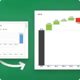
How to Print Excel Worksheets with Gridlines

Because they don’t print by default, we’ll show you how to print Excel worksheets with gridlines using both the desktop application and Microsoft Excel on the web.

If you’re printing an Excel spreadsheet with a lot of data, you may want to include the gridlines. These provide you with subtle borders around your cells without having to manually add them, thus making the data easier to read.

Gridlines Versus Cell Borders in Excel

The advantage to using gridlines versus cell borders when you print in Excel is that they appear around your data automatically when you mark the option as described below.

By default, the gridlines encompass only the data in your sheet. This means if you add or remove data later, the gridlines automatically accommodate those changes.

When you apply cell borders to your data for printing instead, those lines do not update automatically. So, if you add or remove data later, you must manually adjust those cell borders before printing.

If you do add cell borders to your sheet for another reason and also want to print the gridlines, both display when you print the sheet. The borders you apply simply appear as bolder lines when you print (or in color per your border settings) as shown below.

Excel print preview with borders and gridlines

How to Print Excel With Gridlines on Desktop

You can print gridlines in Excel on Windows and Mac by adjusting the same setting. However, Excel on Windows does provide another way to add gridlines when you’re ready to print.

Open your Excel workbook on Windows or Mac to the sheet you want to print.
Go to the Page Layout tab and check the box next to Print in the Gridlines section.

Print checkbox for Gridlines on the Page Layout tab

To see a preview or print the sheet, head to the File tab and pick Print . You’ll see your sheet preview with the gridlines.

If you want to print the entire workbook with gridlines, you’ll need to add them to each individual sheet first by following the above steps.

Display the Gridlines in the Print Preview on Windows

If you forget to mark the Print option for gridlines on the Page Layout tab as described above and are already in the print preview, you can add the lines there if you’re using Excel on Windows.

In the preview, move to the bottom of the print settings and select Page Setup .

Page Setup below the Print Settings in Excel on Windows

Go to the Sheet tab, check the box for Gridlines in the Print section, and choose OK .

Gridlines checkbox in the Page Setup box on Windows

You’ll then see the gridlines in the print preview for the spreadsheet.

Follow these same steps if you want to print other sheets in the workbook with gridlines.

How to Print Excel With Lines on the Web

If you’re using Excel on the web, you can easily print the gridlines for your worksheet.

Visit Excel online , sign in with your Microsoft account, and open the workbook with the sheet you want to print.
Go to the Page Layout tab and pick Page Setup . Alternatively, select File > Print and pick Print .

Page Setup on the Page Layout tab in Excel on the web

On the right side, expand Format options and check the box for Gridlines . You’ll then see the lines displayed on your sheet, adjust any other print settings as needed, and print the spreadsheet.

Like in the desktop application, if you want to print the whole workbook with gridlines, you’ll need to add them to each sheet individually using the above steps.

Gridlines for Easy Reading in Excel

Not only can printing your sheet with gridlines in Excel save you time from manually adding cell borders, but gridlines can accommodate any changes you make to your data automatically. Plus, they make your printed data easier to read.

Now that you know how to print in Excel with lines, look at how to get rid of dotted lines in Excel too.

Sandy Writtenhouse is a freelance technology writer and former Project, Department, and Program Manager. She turned her education, job experience, and love of technology into a full-time writing career. With all sorts of gadgets in her home and her hands, she seeks to help others make life easier through technology. Read Sandy's Full Bio

How to Print Gridlines in Excel?

Gridlines in Excel are the light-colored lines that surround every cell of your spreadsheet. These lines help to demarcate the area occupied by a cell and thus improve the readability of your data.

However, when you print your spreadsheet, you will notice that, by default, the grid lines don’t appear in the printout .

If you want the gridlines to appear on your printed sheet, you will need to manually set them.

In this tutorial, I will show you three easy ways in which you can print gridlines in Excel :

Using the Sheet Options group
Using the Page Setup launcher
From the Print Preview mode

Table of Contents

How to Print Gridlines in Excel

Let us say you want to print the following dataset:

Dataset with Gridlines that need to be printed

Notice the absence of any cell borders . The light-colored lines separating the cells are the gridlines .

When you try to print this dataset out on a paper, you’re probably going to get something that looks like this:

The printout does not have any grid lines separating the cells, so it is hard to tell the rows apart. It gets even harder when you have larger datasets with multiple rows of data.

So, let us see three ways to make sure the gridlines get printed along with the data.

Method 1: Printing Gridlines using Sheet Options

The easiest and quickest way to add gridlines to your printouts is using the ‘ Sheet Options ’ group. Here are the steps to add gridlines to your page using this method:

This group contains two options, one for the Gridlines and another for the Headings .

Make sure the checkbox next to ‘Print’ is checked

This will make sure that your printouts include gridlines when you decide to print your sheet.

This was one way of adding gridlines to your printouts. Let’s look at other ways.

Method 2: Printing Gridlines using Page Setup Launcher Tool

In this method, we will use a dialog box launcher tool ( ). This is a tiny icon that appears in a group. It provides a shortcut to open dialog boxes or task panes related to a particular group.

If you want to make sure that gridlines get printed to the page along with your data, you need to open the Page Setup launcher. Here are the steps you need to follow for this:

Select the area of your worksheet that you want to print. You can do this by dragging your mouse to make a box around your print area.

Now, you must be wondering why you should use this Page Setup dialog box method instead of the first method, where you can simply check the box in the ribbon itself and then print with gridlines.

If all you want to do is enable printing of the gridlines, use the first method (it’s faster).

With this second method (of using the Page Setup dialog box), you also get access to many other options that you may want to use while printing your work (such as repeating the headers or changing the print layout or print row numbers )

Method 3: Printing Guidelines from Print Preview Mode

If your page is already set to print and you see from the preview on the right-hand side that the page does not show any gridlines, then you can directly reach the Page Setup dialog box from there.

Here’s how to add gridlines to your page directly from Print mode:

If you’re not already in Print preview mode, then press CTRL+P (if you’re on a Mac, press Cmd+P), or navigate to File->Print . This will bring you to Print Preview mode.

Page Setup option in the print preview window

This will open the Page Setup dialog box.
Click OK to close the Page Setup dialog box.

If you’re ready to print now, you can go ahead and press the large Print button on the left-hand side.

Troubleshooting Printing Issues When Printing Gridlines

The gridlines typically get printed only around your actual data. If you want the gridlines around empty cells too, then you need to set the print area to include those cells.

If you still have trouble printing gridlines after trying all three methods mentioned in this tutorial, you can try one of the following:

Launch the Page Setup dialog box
Select the Sheet tab

Click OK to close the dialog box.
Check if there are any issues with the printer driver. You can try downloading the latest driver from the printer manufacturer’s website.
Select the range of cells you want the borders around.
Select the Home tab.

In this tutorial, we demonstrated three ways in which you can print gridlines in Excel.

We hope you found these tips helpful in improving the readability and look of your pages when printed.

Show or hide gridlines on a worksheet

About gridlines

Hide gridlines on a worksheet

Show gridlines on a worksheet

Need more help?

Was this information helpful?

3 Easy Ways Add Grid Lines to Your Excel Spreadsheet

Enabling Gridlines (Windows)

Showing Gridlines in Excel for Windows

Expert Q&A

You Might Also Like

About This Article

Is this article up to date?

Featured Articles

Trending Articles

Watch Articles

How to show and hide gridlines in Excel

Show gridlines in Excel

Show / hide gridlines in Excel by changing the fill color

Make Excel hide gridlines only in specific cells

Remove gridlines by changing their color

You may also be interested in

55 comments

7 Ways to Add or Remove Gridlines in Microsoft Excel

Add or Remove Gridlines from the View Tab

Add or Remove Gridlines from the Excel Options Menu

Add or Remove Gridlines with a Keyboard Shortcut

Add or Remove Gridlines from the Quick Access Toolbar

Add or Remove Gridlines when Printing

Add or Remove Gridlines from All Sheets with VBA

Add or Remove Gridlines from All Sheets with Office Scripts

Conclusions

About the Author

John MacDougall

Related Posts

What is an Absolute Reference in Excel?

What Does $ Mean in Excel?

7 Way to Unprotect a Sheet in Microsoft Excel

Get the Latest Microsoft Excel Tips

Working with Gridlines in Excel: How to Add, Remove, Change, and Print Gridlines

Working with Gridlines in Excel

How to Remove Gridlines in Excel Worksheets

How to Show Gridlines in a Specific Area in the Worksheet

Changing the Color of the Gridlines in Excel

Printing the Gridlines in Excel

Leave a Comment Cancel reply

How to Remove or Add Gridlines in Excel

In This Article

What Are Gridlines and How Do They Work?

Change the Fill Color to Remove Excel Gridlines

Change the Color of Excel Gridlines for the Whole Worksheet

How to Hide Gridlines for Particular Columns and Rows

How to Turn Gridlines On and Off for the Whole Worksheet

How to Show or Hide Gridlines in Excel

Show or Hide Gridlines in Excel Worksheets (+ Shortcuts)

Hide or remove gridlines

Subscribe to get more articles like this one

More resources

Related courses

You may also like

What is Power Query in Excel?

How to Stop or Control Green Error Checking Markers in Excel

Excel Shortcuts to Zoom In and Out in Your Worksheets (4 Shortcuts)

Our Courses

Privacy Overview

Edit Gridlines in Excel (Add, Remove, Change, and Print)

Removing Gridlines in Excel Worksheets

Showing Gridlines in Specific Area in Worksheet

Changing Color of Gridlines in Excel

Printing Gridlines in Excel

Controlling Chart Gridlines in Excel

Showing Single or Multiple Gridlines in Excel Chart

Things to Remember

Frequently Asked Questions

Edit Gridlines in Excel: Knowledge Hub

What is ExcelDemy?

Leave a reply Cancel reply

How to Add Gridlines in Excel

Step 1: Open the Worksheet

Step 2: Select the Cells