assignment problem of maximization

Hungarian Method

The Hungarian method is a computational optimization technique that addresses the assignment problem in polynomial time and foreshadows following primal-dual alternatives. In 1955, Harold Kuhn used the term “Hungarian method” to honour two Hungarian mathematicians, Dénes Kőnig and Jenő Egerváry. Let’s go through the steps of the Hungarian method with the help of a solved example.

Hungarian Method to Solve Assignment Problems

The Hungarian method is a simple way to solve assignment problems. Let us first discuss the assignment problems before moving on to learning the Hungarian method.

What is an Assignment Problem?

A transportation problem is a type of assignment problem. The goal is to allocate an equal amount of resources to the same number of activities. As a result, the overall cost of allocation is minimised or the total profit is maximised.

Because available resources such as workers, machines, and other resources have varying degrees of efficiency for executing different activities, and hence the cost, profit, or loss of conducting such activities varies.

Assume we have ‘n’ jobs to do on ‘m’ machines (i.e., one job to one machine). Our goal is to assign jobs to machines for the least amount of money possible (or maximum profit). Based on the notion that each machine can accomplish each task, but at variable levels of efficiency.

Hungarian Method Steps

Check to see if the number of rows and columns are equal; if they are, the assignment problem is considered to be balanced. Then go to step 1. If it is not balanced, it should be balanced before the algorithm is applied.

Step 1 – In the given cost matrix, subtract the least cost element of each row from all the entries in that row. Make sure that each row has at least one zero.

Step 2 – In the resultant cost matrix produced in step 1, subtract the least cost element in each column from all the components in that column, ensuring that each column contains at least one zero.

Step 3 – Assign zeros

• Analyse the rows one by one until you find a row with precisely one unmarked zero. Encircle this lonely unmarked zero and assign it a task. All other zeros in the column of this circular zero should be crossed out because they will not be used in any future assignments. Continue in this manner until you’ve gone through all of the rows.
• Examine the columns one by one until you find one with precisely one unmarked zero. Encircle this single unmarked zero and cross any other zero in its row to make an assignment to it. Continue until you’ve gone through all of the columns.

Step 4 – Perform the Optimal Test

• The present assignment is optimal if each row and column has exactly one encircled zero.
• The present assignment is not optimal if at least one row or column is missing an assignment (i.e., if at least one row or column is missing one encircled zero). Continue to step 5. Subtract the least cost element from all the entries in each column of the final cost matrix created in step 1 and ensure that each column has at least one zero.

Step 5 – Draw the least number of straight lines to cover all of the zeros as follows:

(a) Highlight the rows that aren’t assigned.

(b) Label the columns with zeros in marked rows (if they haven’t already been marked).

(c) Highlight the rows that have assignments in indicated columns (if they haven’t previously been marked).

(d) Continue with (b) and (c) until no further marking is needed.

(f) Simply draw the lines through all rows and columns that are not marked. If the number of these lines equals the order of the matrix, then the solution is optimal; otherwise, it is not.

Step 6 – Find the lowest cost factor that is not covered by the straight lines. Subtract this least-cost component from all the uncovered elements and add it to all the elements that are at the intersection of these straight lines, but leave the rest of the elements alone.

Step 7 – Continue with steps 1 – 6 until you’ve found the highest suitable assignment.

Hungarian Method Example

Use the Hungarian method to solve the given assignment problem stated in the table. The entries in the matrix represent each man’s processing time in hours.

\(\begin{array}{l}\begin{bmatrix} & I & II & III & IV & V \\1 & 20 & 15 & 18 & 20 & 25 \\2 & 18 & 20 & 12 & 14 & 15 \\3 & 21 & 23 & 25 & 27 & 25 \\4 & 17 & 18 & 21 & 23 & 20 \\5 & 18 & 18 & 16 & 19 & 20 \\\end{bmatrix}\end{array} \)

With 5 jobs and 5 men, the stated problem is balanced.

\(\begin{array}{l}A = \begin{bmatrix}20 & 15 & 18 & 20 & 25 \\18 & 20 & 12 & 14 & 15 \\21 & 23 & 25 & 27 & 25 \\17 & 18 & 21 & 23 & 20 \\18 & 18 & 16 & 19 & 20 \\\end{bmatrix}\end{array} \)

Subtract the lowest cost element in each row from all of the elements in the given cost matrix’s row. Make sure that each row has at least one zero.

\(\begin{array}{l}A = \begin{bmatrix}5 & 0 & 3 & 5 & 10 \\6 & 8 & 0 & 2 & 3 \\0 & 2 & 4 & 6 & 4 \\0 & 1 & 4 & 6 & 3 \\2 & 2 & 0 & 3 & 4 \\\end{bmatrix}\end{array} \)

Subtract the least cost element in each Column from all of the components in the given cost matrix’s Column. Check to see if each column has at least one zero.

\(\begin{array}{l}A = \begin{bmatrix}5 & 0 & 3 & 3 & 7 \\6 & 8 & 0 & 0 & 0 \\0 & 2 & 4 & 4 & 1 \\0 & 1 & 4 & 4 & 0 \\2 & 2 & 0 & 1 & 1 \\\end{bmatrix}\end{array} \)

When the zeros are assigned, we get the following:

The present assignment is optimal because each row and column contain precisely one encircled zero.

Where 1 to II, 2 to IV, 3 to I, 4 to V, and 5 to III are the best assignments.

Hence, z = 15 + 14 + 21 + 20 + 16 = 86 hours is the optimal time.

Practice Question on Hungarian Method

Use the Hungarian method to solve the following assignment problem shown in table. The matrix entries represent the time it takes for each job to be processed by each machine in hours.

\(\begin{array}{l}\begin{bmatrix}J/M & I & II & III & IV & V \\1 & 9 & 22 & 58 & 11 & 19 \\2 & 43 & 78 & 72 & 50 & 63 \\3 & 41 & 28 & 91 & 37 & 45 \\4 & 74 & 42 & 27 & 49 & 39 \\5 & 36 & 11 & 57 & 22 & 25 \\\end{bmatrix}\end{array} \)

Stay tuned to BYJU’S – The Learning App and download the app to explore all Maths-related topics.

Frequently Asked Questions on Hungarian Method

What is hungarian method.

The Hungarian method is defined as a combinatorial optimization technique that solves the assignment problems in polynomial time and foreshadowed subsequent primal–dual approaches.

What are the steps involved in Hungarian method?

The following is a quick overview of the Hungarian method: Step 1: Subtract the row minima. Step 2: Subtract the column minimums. Step 3: Use a limited number of lines to cover all zeros. Step 4: Add some more zeros to the equation.

What is the purpose of the Hungarian method?

When workers are assigned to certain activities based on cost, the Hungarian method is beneficial for identifying minimum costs.

Leave a Comment Cancel reply

Your Mobile number and Email id will not be published. Required fields are marked *

Request OTP on Voice Call

Post My Comment

Register with BYJU'S & Download Free PDFs

Register with byju's & watch live videos.

4.7 Applied Optimization Problems

Learning objectives.

• 4.7.1 Set up and solve optimization problems in several applied fields.

One common application of calculus is calculating the minimum or maximum value of a function. For example, companies often want to minimize production costs or maximize revenue. In manufacturing, it is often desirable to minimize the amount of material used to package a product with a certain volume. In this section, we show how to set up these types of minimization and maximization problems and solve them by using the tools developed in this chapter.

Solving Optimization Problems over a Closed, Bounded Interval

The basic idea of the optimization problems that follow is the same. We have a particular quantity that we are interested in maximizing or minimizing. However, we also have some auxiliary condition that needs to be satisfied. For example, in Example 4.32 , we are interested in maximizing the area of a rectangular garden. Certainly, if we keep making the side lengths of the garden larger, the area will continue to become larger. However, what if we have some restriction on how much fencing we can use for the perimeter? In this case, we cannot make the garden as large as we like. Let’s look at how we can maximize the area of a rectangle subject to some constraint on the perimeter.

Example 4.32

Maximizing the area of a garden.

A rectangular garden is to be constructed using a rock wall as one side of the garden and wire fencing for the other three sides ( Figure 4.62 ). Given 100 100 ft of wire fencing, determine the dimensions that would create a garden of maximum area. What is the maximum area?

Let x x denote the length of the side of the garden perpendicular to the rock wall and y y denote the length of the side parallel to the rock wall. Then the area of the garden is

We want to find the maximum possible area subject to the constraint that the total fencing is 100 ft . 100 ft . From Figure 4.62 , the total amount of fencing used will be 2 x + y . 2 x + y . Therefore, the constraint equation is

Solving this equation for y , y , we have y = 100 − 2 x . y = 100 − 2 x . Thus, we can write the area as

Before trying to maximize the area function A ( x ) = 100 x − 2 x 2 , A ( x ) = 100 x − 2 x 2 , we need to determine the domain under consideration. To construct a rectangular garden, we certainly need the lengths of both sides to be positive. Therefore, we need x > 0 x > 0 and y > 0 . y > 0 . Since y = 100 − 2 x , y = 100 − 2 x , if y > 0 , y > 0 , then x < 50 . x < 50 . Therefore, we are trying to determine the maximum value of A ( x ) A ( x ) for x x over the open interval ( 0 , 50 ) . ( 0 , 50 ) . We do not know that a function necessarily has a maximum value over an open interval. However, we do know that a continuous function has an absolute maximum (and absolute minimum) over a closed interval. Therefore, let’s consider the function A ( x ) = 100 x − 2 x 2 A ( x ) = 100 x − 2 x 2 over the closed interval [ 0 , 50 ] . [ 0 , 50 ] . If the maximum value occurs at an interior point, then we have found the value x x in the open interval ( 0 , 50 ) ( 0 , 50 ) that maximizes the area of the garden. Therefore, we consider the following problem:

Maximize A ( x ) = 100 x − 2 x 2 A ( x ) = 100 x − 2 x 2 over the interval [ 0 , 50 ] . [ 0 , 50 ] .

As mentioned earlier, since A A is a continuous function on a closed, bounded interval, by the extreme value theorem, it has a maximum and a minimum. These extreme values occur either at endpoints or critical points. At the endpoints, A ( x ) = 0 . A ( x ) = 0 . Since the area is positive for all x x in the open interval ( 0 , 50 ) , ( 0 , 50 ) , the maximum must occur at a critical point. Differentiating the function A ( x ) , A ( x ) , we obtain

Therefore, the only critical point is x = 25 x = 25 ( Figure 4.63 ). We conclude that the maximum area must occur when x = 25 . x = 25 . Then we have y = 100 − 2 x = 100 − 2 ( 25 ) = 50 . y = 100 − 2 x = 100 − 2 ( 25 ) = 50 . To maximize the area of the garden, let x = 25 x = 25 ft and y = 50 ft . y = 50 ft . The area of this garden is 1250 ft 2 . 1250 ft 2 .

Checkpoint 4.31

Determine the maximum area if we want to make the same rectangular garden as in Figure 4.63 , but we have 200 200 ft of fencing.

Now let’s look at a general strategy for solving optimization problems similar to Example 4.32 .

Problem-Solving Strategy

Problem-solving strategy: solving optimization problems.

• Introduce all variables. If applicable, draw a figure and label all variables.
• Determine which quantity is to be maximized or minimized, and for what range of values of the other variables (if this can be determined at this time).
• Write a formula for the quantity to be maximized or minimized in terms of the variables. This formula may involve more than one variable.
• Write any equations relating the independent variables in the formula from step 3 . 3 . Use these equations to write the quantity to be maximized or minimized as a function of one variable.
• Identify the domain of consideration for the function in step 4 4 based on the physical problem to be solved.
• Locate the maximum or minimum value of the function from step 4 . 4 . This step typically involves looking for critical points and evaluating a function at endpoints.

Now let’s apply this strategy to maximize the volume of an open-top box given a constraint on the amount of material to be used.

Example 4.33

Maximizing the volume of a box.

An open-top box is to be made from a 24 24 in. by 36 36 in. piece of cardboard by removing a square from each corner of the box and folding up the flaps on each side. What size square should be cut out of each corner to get a box with the maximum volume?

Step 1: Let x x be the side length of the square to be removed from each corner ( Figure 4.64 ). Then, the remaining four flaps can be folded up to form an open-top box. Let V V be the volume of the resulting box.

Step 2: We are trying to maximize the volume of a box. Therefore, the problem is to maximize V . V .

Step 3: As mentioned in step 2 , 2 , we are trying to maximize the volume of a box. The volume of a box is V = L · W · H , V = L · W · H , where L , W , and H L , W , and H are the length, width, and height, respectively.

Step 4: From Figure 4.64 , we see that the height of the box is x x inches, the length is 36 − 2 x 36 − 2 x inches, and the width is 24 − 2 x 24 − 2 x inches. Therefore, the volume of the box is

Step 5: To determine the domain of consideration, let’s examine Figure 4.64 . Certainly, we need x > 0 . x > 0 . Furthermore, the side length of the square cannot be greater than or equal to half the length of the shorter side, 24 24 in.; otherwise, one of the flaps would be completely cut off. Therefore, we are trying to determine whether there is a maximum volume of the box for x x over the open interval ( 0 , 12 ) . ( 0 , 12 ) . Since V V is a continuous function over the closed interval [ 0 , 12 ] , [ 0 , 12 ] , we know V V will have an absolute maximum over the closed interval. Therefore, we consider V V over the closed interval [ 0 , 12 ] [ 0 , 12 ] and check whether the absolute maximum occurs at an interior point.

Step 6: Since V ( x ) V ( x ) is a continuous function over the closed, bounded interval [ 0 , 12 ] , [ 0 , 12 ] , V V must have an absolute maximum (and an absolute minimum). Since V ( x ) = 0 V ( x ) = 0 at the endpoints and V ( x ) > 0 V ( x ) > 0 for 0 < x < 12 , 0 < x < 12 , the maximum must occur at a critical point. The derivative is

To find the critical points, we need to solve the equation

Dividing both sides of this equation by 12 , 12 , the problem simplifies to solving the equation

Using the quadratic formula, we find that the critical points are

Since 10 + 2 7 10 + 2 7 is not in the domain of consideration, the only critical point we need to consider is 10 − 2 7 . 10 − 2 7 . Therefore, the volume is maximized if we let x = 10 − 2 7 in . x = 10 − 2 7 in . The maximum volume is V ( 10 − 2 7 ) = 640 + 448 7 ≈ 1825 in . 3 V ( 10 − 2 7 ) = 640 + 448 7 ≈ 1825 in . 3 as shown in the following graph.

Watch a video about optimizing the volume of a box.

Checkpoint 4.32

Suppose the dimensions of the cardboard in Example 4.33 are 20 in. by 30 in. Let x x be the side length of each square and write the volume of the open-top box as a function of x . x . Determine the domain of consideration for x . x .

Example 4.34

Minimizing travel time.

An island is 2 mi 2 mi due north of its closest point along a straight shoreline. A visitor is staying at a cabin on the shore that is 6 mi 6 mi west of that point. The visitor is planning to go from the cabin to the island. Suppose the visitor runs at a rate of 8 mph 8 mph and swims at a rate of 3 mph . 3 mph . How far should the visitor run before swimming to minimize the time it takes to reach the island?

Step 1: Let x x be the distance running and let y y be the distance swimming ( Figure 4.66 ). Let T T be the time it takes to get from the cabin to the island.

Step 2: The problem is to minimize T . T .

Step 3: To find the time spent traveling from the cabin to the island, add the time spent running and the time spent swimming. Since Distance = = Rate × × Time ( D = R × T ) , ( D = R × T ) , the time spent running is

and the time spent swimming is

Therefore, the total time spent traveling is

Step 4: From Figure 4.66 , the line segment of y y miles forms the hypotenuse of a right triangle with legs of length 2 mi 2 mi and 6 − x mi . 6 − x mi . Therefore, by the Pythagorean theorem, 2 2 + ( 6 − x ) 2 = y 2 , 2 2 + ( 6 − x ) 2 = y 2 , and we obtain y = ( 6 − x ) 2 + 4 . y = ( 6 − x ) 2 + 4 . Thus, the total time spent traveling is given by the function

Step 5: From Figure 4.66 , we see that 0 ≤ x ≤ 6 . 0 ≤ x ≤ 6 . Therefore, [ 0 , 6 ] [ 0 , 6 ] is the domain of consideration.

Step 6: Since T ( x ) T ( x ) is a continuous function over a closed, bounded interval, it has a maximum and a minimum. Let’s begin by looking for any critical points of T T over the interval [ 0 , 6 ] . [ 0 , 6 ] . The derivative is

If T ′ ( x ) = 0 , T ′ ( x ) = 0 , then

Squaring both sides of this equation, we see that if x x satisfies this equation, then x x must satisfy

which implies

We conclude that if x x is a critical point, then x x satisfies

Therefore, the possibilities for critical points are

Since x = 6 + 6 / 55 x = 6 + 6 / 55 is not in the domain, it is not a possibility for a critical point. On the other hand, x = 6 − 6 / 55 x = 6 − 6 / 55 is in the domain. Since we squared both sides of Equation 4.6 to arrive at the possible critical points, it remains to verify that x = 6 − 6 / 55 x = 6 − 6 / 55 satisfies Equation 4.6 . Since x = 6 − 6 / 55 x = 6 − 6 / 55 does satisfy that equation, we conclude that x = 6 − 6 / 55 x = 6 − 6 / 55 is a critical point, and it is the only one. To justify that the time is minimized for this value of x , x , we just need to check the values of T ( x ) T ( x ) at the endpoints x = 0 x = 0 and x = 6 , x = 6 , and compare them with the value of T ( x ) T ( x ) at the critical point x = 6 − 6 / 55 . x = 6 − 6 / 55 . We find that T ( 0 ) ≈ 2.108 h T ( 0 ) ≈ 2.108 h and T ( 6 ) ≈ 1.417 h, T ( 6 ) ≈ 1.417 h, whereas T ( 6 − 6 / 55 ) ≈ 1.368 h . T ( 6 − 6 / 55 ) ≈ 1.368 h . Therefore, we conclude that T T has a local minimum at x ≈ 5.19 x ≈ 5.19 mi.

Checkpoint 4.33

Suppose the island is 1 1 mi from shore, and the distance from the cabin to the point on the shore closest to the island is 15 mi . 15 mi . Suppose a visitor swims at the rate of 2.5 mph 2.5 mph and runs at a rate of 6 mph . 6 mph . Let x x denote the distance the visitor will run before swimming, and find a function for the time it takes the visitor to get from the cabin to the island.

In business, companies are interested in maximizing revenue . In the following example, we consider a scenario in which a company has collected data on how many cars it is able to lease, depending on the price it charges its customers to rent a car. Let’s use these data to determine the price the company should charge to maximize the amount of money it brings in.

Example 4.35

Maximizing revenue.

Owners of a car rental company have determined that if they charge customers p p dollars per day to rent a car, where 50 ≤ p ≤ 200 , 50 ≤ p ≤ 200 , the number of cars n n they rent per day can be modeled by the linear function n ( p ) = 1000 − 5 p . n ( p ) = 1000 − 5 p . If they charge $ 50 $ 50 per day or less, they will rent all their cars. If they charge $ 200 $ 200 per day or more, they will not rent any cars. Assuming the owners plan to charge customers between $50 per day and $ 200 $ 200 per day to rent a car, how much should they charge to maximize their revenue?

Step 1: Let p p be the price charged per car per day and let n n be the number of cars rented per day. Let R R be the revenue per day.

Step 2: The problem is to maximize R . R .

Step 3: The revenue (per day) is equal to the number of cars rented per day times the price charged per car per day—that is, R = n × p . R = n × p .

Step 4: Since the number of cars rented per day is modeled by the linear function n ( p ) = 1000 − 5 p , n ( p ) = 1000 − 5 p , the revenue R R can be represented by the function

Step 5: Since the owners plan to charge between $ 50 $ 50 per car per day and $ 200 $ 200 per car per day, the problem is to find the maximum revenue R ( p ) R ( p ) for p p in the closed interval [ 50 , 200 ] . [ 50 , 200 ] .

Step 6: Since R R is a continuous function over the closed, bounded interval [ 50 , 200 ] , [ 50 , 200 ] , it has an absolute maximum (and an absolute minimum) in that interval. To find the maximum value, look for critical points. The derivative is R ′ ( p ) = −10 p + 1000 . R ′ ( p ) = −10 p + 1000 . Therefore, the critical point is p = 100 p = 100 When p = 100 , p = 100 , R ( 100 ) = $ 50,000 . R ( 100 ) = $ 50,000 . When p = 50 , p = 50 , R ( p ) = $ 37,500 . R ( p ) = $ 37,500 . When p = 200 , p = 200 , R ( p ) = $ 0 . R ( p ) = $ 0 . Therefore, the absolute maximum occurs at p = $ 100 . p = $ 100 . The car rental company should charge $ 100 $ 100 per day per car to maximize revenue as shown in the following figure.

Checkpoint 4.34

A car rental company charges its customers p p dollars per day, where 60 ≤ p ≤ 150 . 60 ≤ p ≤ 150 . It has found that the number of cars rented per day can be modeled by the linear function n ( p ) = 750 − 5 p . n ( p ) = 750 − 5 p . How much should the company charge each customer to maximize revenue?

Example 4.36

Maximizing the area of an inscribed rectangle.

A rectangle is to be inscribed in the ellipse

What should the dimensions of the rectangle be to maximize its area? What is the maximum area?

Step 1: For a rectangle to be inscribed in the ellipse, the sides of the rectangle must be parallel to the axes. Let L L be the length of the rectangle and W W be its width. Let A A be the area of the rectangle.

Step 2: The problem is to maximize A . A .

Step 3: The area of the rectangle is A = L W . A = L W .

Step 4: Let ( x , y ) ( x , y ) be the corner of the rectangle that lies in the first quadrant, as shown in Figure 4.68 . We can write length L = 2 x L = 2 x and width W = 2 y . W = 2 y . Since x 2 4 + y 2 = 1 x 2 4 + y 2 = 1 and y > 0 , y > 0 , we have y = 1 − x 2 4 . y = 1 − x 2 4 . Therefore, the area is

Step 5: From Figure 4.68 , we see that to inscribe a rectangle in the ellipse, the x x -coordinate of the corner in the first quadrant must satisfy 0 < x < 2 . 0 < x < 2 . Therefore, the problem reduces to looking for the maximum value of A ( x ) A ( x ) over the open interval ( 0 , 2 ) . ( 0 , 2 ) . Since A ( x ) A ( x ) will have an absolute maximum (and absolute minimum) over the closed interval [ 0 , 2 ] , [ 0 , 2 ] , we consider A ( x ) = 2 x 4 − x 2 A ( x ) = 2 x 4 − x 2 over the interval [ 0 , 2 ] . [ 0 , 2 ] . If the absolute maximum occurs at an interior point, then we have found an absolute maximum in the open interval.

Step 6: As mentioned earlier, A ( x ) A ( x ) is a continuous function over the closed, bounded interval [ 0 , 2 ] . [ 0 , 2 ] . Therefore, it has an absolute maximum (and absolute minimum). At the endpoints x = 0 x = 0 and x = 2 , x = 2 , A ( x ) = 0 . A ( x ) = 0 . For 0 < x < 2 , 0 < x < 2 , A ( x ) > 0 . A ( x ) > 0 . Therefore, the maximum must occur at a critical point. Taking the derivative of A ( x ) , A ( x ) , we obtain

To find critical points, we need to find where A ′ ( x ) = 0 . A ′ ( x ) = 0 . We can see that if x x is a solution of

then x x must satisfy

Therefore, x 2 = 2 . x 2 = 2 . Thus, x = ± 2 x = ± 2 are the possible solutions of Equation 4.7 . Since we are considering x x over the interval [ 0 , 2 ] , [ 0 , 2 ] , x = 2 x = 2 is a possibility for a critical point, but x = − 2 x = − 2 is not. Therefore, we check whether 2 2 is a solution of Equation 4.7 . Since x = 2 x = 2 is a solution of Equation 4.7 , we conclude that 2 2 is the only critical point of A ( x ) A ( x ) in the interval [ 0 , 2 ] . [ 0 , 2 ] . Therefore, A ( x ) A ( x ) must have an absolute maximum at the critical point x = 2 . x = 2 . To determine the dimensions of the rectangle, we need to find the length L L and the width W . W . If x = 2 x = 2 then

Therefore, the dimensions of the rectangle are L = 2 x = 2 2 L = 2 x = 2 2 and W = 2 y = 2 2 = 2 . W = 2 y = 2 2 = 2 . The area of this rectangle is A = L W = ( 2 2 ) ( 2 ) = 4 . A = L W = ( 2 2 ) ( 2 ) = 4 .

Checkpoint 4.35

Modify the area function A A if the rectangle is to be inscribed in the unit circle x 2 + y 2 = 1 . x 2 + y 2 = 1 . What is the domain of consideration?

Solving Optimization Problems when the Interval Is Not Closed or Is Unbounded

In the previous examples, we considered functions on closed, bounded domains. Consequently, by the extreme value theorem, we were guaranteed that the functions had absolute extrema. Let’s now consider functions for which the domain is neither closed nor bounded.

Many functions still have at least one absolute extrema, even if the domain is not closed or the domain is unbounded. For example, the function f ( x ) = x 2 + 4 f ( x ) = x 2 + 4 over ( − ∞ , ∞ ) ( − ∞ , ∞ ) has an absolute minimum of 4 4 at x = 0 . x = 0 . Therefore, we can still consider functions over unbounded domains or open intervals and determine whether they have any absolute extrema. In the next example, we try to minimize a function over an unbounded domain. We will see that, although the domain of consideration is ( 0 , ∞ ) , ( 0 , ∞ ) , the function has an absolute minimum.

In the following example, we look at constructing a box of least surface area with a prescribed volume. It is not difficult to show that for a closed-top box, by symmetry, among all boxes with a specified volume, a cube will have the smallest surface area. Consequently, we consider the modified problem of determining which open-topped box with a specified volume has the smallest surface area.

Example 4.37

Minimizing surface area.

A rectangular box with a square base, an open top, and a volume of 216 216 in. 3 is to be constructed. What should the dimensions of the box be to minimize the surface area of the box? What is the minimum surface area?

Step 1: Draw a rectangular box and introduce the variable x x to represent the length of each side of the square base; let y y represent the height of the box. Let S S denote the surface area of the open-top box.

Step 2: We need to minimize the surface area. Therefore, we need to minimize S . S .

Step 3: Since the box has an open top, we need only determine the area of the four vertical sides and the base. The area of each of the four vertical sides is x · y . x · y . The area of the base is x 2 . x 2 . Therefore, the surface area of the box is

Step 4: Since the volume of this box is x 2 y x 2 y and the volume is given as 216 in . 3 , 216 in . 3 , the constraint equation is

Solving the constraint equation for y , y , we have y = 216 x 2 . y = 216 x 2 . Therefore, we can write the surface area as a function of x x only:

Therefore, S ( x ) = 864 x + x 2 . S ( x ) = 864 x + x 2 .

Step 5: Since we are requiring that x 2 y = 216 , x 2 y = 216 , we cannot have x = 0 . x = 0 . Therefore, we need x > 0 . x > 0 . On the other hand, x x is allowed to have any positive value. Note that as x x becomes large, the height of the box y y becomes correspondingly small so that x 2 y = 216 . x 2 y = 216 . Similarly, as x x becomes small, the height of the box becomes correspondingly large. We conclude that the domain is the open, unbounded interval ( 0 , ∞ ) . ( 0 , ∞ ) . Note that, unlike the previous examples, we cannot reduce our problem to looking for an absolute maximum or absolute minimum over a closed, bounded interval. However, in the next step, we discover why this function must have an absolute minimum over the interval ( 0 , ∞ ) . ( 0 , ∞ ) .

Step 6: Note that as x → 0 + , x → 0 + , S ( x ) → ∞ . S ( x ) → ∞ . Also, as x → ∞ , x → ∞ , S ( x ) → ∞ . S ( x ) → ∞ . Since S S is a continuous function that approaches infinity at the ends, it must have an absolute minimum at some x ∈ ( 0 , ∞ ) . x ∈ ( 0 , ∞ ) . This minimum must occur at a critical point of S . S . The derivative is

Therefore, S ′ ( x ) = 0 S ′ ( x ) = 0 when 2 x = 864 x 2 . 2 x = 864 x 2 . Solving this equation for x , x , we obtain x 3 = 432 , x 3 = 432 , so x = 432 3 = 6 2 3 . x = 432 3 = 6 2 3 . Since this is the only critical point of S , S , the absolute minimum must occur at x = 6 2 3 x = 6 2 3 (see Figure 4.70 ). When x = 6 2 3 , x = 6 2 3 , y = 216 ( 6 2 3 ) 2 = 3 2 3 in . y = 216 ( 6 2 3 ) 2 = 3 2 3 in . Therefore, the dimensions of the box should be x = 6 2 3 in . x = 6 2 3 in . and y = 3 2 3 in . y = 3 2 3 in . With these dimensions, the surface area is

Checkpoint 4.36

Consider the same open-top box, which is to have volume 216 in . 3 . 216 in . 3 . Suppose the cost of the material for the base is 20 ¢ / in . 2 20 ¢ / in . 2 and the cost of the material for the sides is 30 ¢ / in . 2 30 ¢ / in . 2 and we are trying to minimize the cost of this box. Write the cost as a function of the side lengths of the base. (Let x x be the side length of the base and y y be the height of the box.)

Section 4.7 Exercises

For the following exercises, answer by proof, counterexample, or explanation.

When you find the maximum for an optimization problem, why do you need to check the sign of the derivative around the critical points?

Why do you need to check the endpoints for optimization problems?

True or False . For every continuous nonlinear function, you can find the value x x that maximizes the function.

True or False . For every continuous nonconstant function on a closed, finite domain, there exists at least one x x that minimizes or maximizes the function.

For the following exercises, set up and evaluate each optimization problem.

To carry a suitcase on an airplane, the length + width + + width + height of the box must be less than or equal to 62 in . 62 in . Assuming the base of the suitcase is square, show that the volume is V = h ( 31 − ( 1 2 ) h ) 2 . V = h ( 31 − ( 1 2 ) h ) 2 . What height allows you to have the largest volume?

You are constructing a cardboard box with the dimensions 2 m by 4 m . 2 m by 4 m . You then cut equal-size squares from each corner so you may fold the edges. What are the dimensions of the box with the largest volume?

Find the positive integer that minimizes the sum of the number and its reciprocal.

Find two positive integers such that their sum is 10 , 10 , and minimize and maximize the sum of their squares.

For the following exercises, consider the construction of a pen to enclose an area.

You have 400 ft 400 ft of fencing to construct a rectangular pen for cattle. What are the dimensions of the pen that maximize the area?

You have 800 ft 800 ft of fencing to make a pen for hogs. If you have a river on one side of your property, what is the dimension of the rectangular pen that maximizes the area?

You need to construct a fence around an area of 1600 ft 2 . 1600 ft 2 . What are the dimensions of the rectangular pen to minimize the amount of material needed?

Two poles are connected by a wire that is also connected to the ground. The first pole is 20 ft 20 ft tall and the second pole is 10 ft 10 ft tall. There is a distance of 30 ft 30 ft between the two poles. Where should the wire be anchored to the ground to minimize the amount of wire needed?

[T] You are moving into a new apartment and notice there is a corner where the hallway narrows from 8 ft to 6 ft . 8 ft to 6 ft . What is the length of the longest item that can be carried horizontally around the corner?

A patient’s pulse measures 70 bpm, 80 bpm, then 120 bpm . 70 bpm, 80 bpm, then 120 bpm . To determine an accurate measurement of pulse, the doctor wants to know what value minimizes the expression ( x − 70 ) 2 + ( x − 80 ) 2 + ( x − 120 ) 2 ? ( x − 70 ) 2 + ( x − 80 ) 2 + ( x − 120 ) 2 ? What value minimizes it?

In the previous problem, assume the patient was nervous during the third measurement, so we only weight that value half as much as the others. What is the value that minimizes ( x − 70 ) 2 + ( x − 80 ) 2 + 1 2 ( x − 120 ) 2 ? ( x − 70 ) 2 + ( x − 80 ) 2 + 1 2 ( x − 120 ) 2 ?

You can run at a speed of 6 6 mph and swim at a speed of 3 3 mph and are located on the shore, 4 4 miles east of an island that is 1 1 mile north of the shoreline. How far should you run west to minimize the time needed to reach the island?

For the following problems, consider a lifeguard at a circular pool with diameter 40 m . 40 m . He must reach someone who is drowning on the exact opposite side of the pool, at position C . C . The lifeguard swims with a speed v v and runs around the pool at speed w = 3 v . w = 3 v .

Find a function that measures the total amount of time it takes to reach the drowning person as a function of the swim angle, θ . θ .

Find at what angle θ θ the lifeguard should swim to reach the drowning person in the least amount of time.

A truck uses gas as g ( v ) = a v + b v , g ( v ) = a v + b v , where v v represents the speed of the truck and g g represents the gallons of fuel per mile. Assuming a a and b b are positive, at what speed is fuel consumption minimized?

For the following exercises, consider a limousine that gets m ( v ) = ( 120 − 2 v ) 5 mi/gal m ( v ) = ( 120 − 2 v ) 5 mi/gal at speed v , v , the chauffeur costs $15/h , $15/h , and gas is $ 3.5 / gal . $ 3.5 / gal .

Find the cost per mile at speed v . v .

Find the cheapest driving speed.

For the following exercises, consider a pizzeria that sell pizzas for a revenue of R ( x ) = a x R ( x ) = a x and costs C ( x ) = b + c x + d x 2 , C ( x ) = b + c x + d x 2 , where x x represents the number of pizzas ;   a   >   c ;   a   >   c .

Find the profit function for the number of pizzas. How many pizzas gives the largest profit per pizza?

Assume that R ( x ) = 10 x R ( x ) = 10 x and C ( x ) = 2 x + x 2 . C ( x ) = 2 x + x 2 . How many pizzas sold maximizes the profit?

Assume that R ( x ) = 15 x , R ( x ) = 15 x , and C ( x ) = 60 + 3 x + 1 2 x 2 . C ( x ) = 60 + 3 x + 1 2 x 2 . How many pizzas sold maximizes the profit?

For the following exercises, consider a wire 4 ft 4 ft long cut into two pieces. One piece forms a circle with radius r r and the other forms a square of side x . x .

Choose x x to maximize the sum of their areas.

Choose x x to minimize the sum of their areas.

For the following exercises, consider two nonnegative numbers x x and y y such that x + y = 10 . x + y = 10 . Maximize and minimize the quantities.

x 2 y 2 x 2 y 2

y − 1 x y − 1 x

x 2 − y x 2 − y

For the following exercises, draw the given optimization problem and solve.

Find the volume of the largest right circular cylinder that fits in a sphere of radius 1 . 1 .

Find the volume of the largest right cone that fits in a sphere of radius 1 . 1 .

Find the area of the largest rectangle that fits into the triangle with sides x = 0 , y = 0 x = 0 , y = 0 and x 4 + y 6 = 1 . x 4 + y 6 = 1 .

Find the largest volume of a cylinder that fits into a cone that has base radius R R and height h . h .

Find the dimensions of the closed cylinder volume V = 16 π V = 16 π that has the least amount of surface area.

Find the dimensions of a right cone with surface area S = 4 π S = 4 π that has the largest volume.

For the following exercises, consider the points on the given graphs. Use a calculator to graph the functions.

[T] Where is the line y = 5 − 2 x y = 5 − 2 x closest to the origin?

[T] Where is the line y = 5 − 2 x y = 5 − 2 x closest to point ( 1 , 1 ) ? ( 1 , 1 ) ?

[T] Where is the parabola y = x 2 y = x 2 closest to point ( 2 , 0 ) ? ( 2 , 0 ) ?

[T] Where is the parabola y = x 2 y = x 2 closest to point ( 0 , 3 ) ? ( 0 , 3 ) ?

For the following exercises, set up, but do not evaluate, each optimization problem.

A window is composed of a semicircle placed on top of a rectangle. If you have 20 ft 20 ft of window-framing materials for the outer frame, what is the maximum size of the window you can create? Use r r to represent the radius of the semicircle.

You have a garden row of 20 20 watermelon plants that produce an average of 30 30 watermelons apiece. For any additional watermelon plants planted, the output per watermelon plant drops by one watermelon. How many extra watermelon plants should you plant?

You are constructing a box for your cat to sleep in. The plush material for the square bottom of the box costs $ 5 / ft 2 $ 5 / ft 2 and the material for the sides costs $ 2 / ft 2 . $ 2 / ft 2 . You need a box with volume 4 ft 3 . 4 ft 3 . Find the dimensions of the box that minimize cost. Use x x to represent the length of the side of the box.

You are building five identical pens adjacent to each other with a total area of 1000 m 2 , 1000 m 2 , as shown in the following figure. What dimensions should you use to minimize the amount of fencing?

You are the manager of an apartment complex with 50 50 units. When you set rent at $ 800 / month, $ 800 / month, all apartments are rented. As you increase rent by $ 25 / month, $ 25 / month, one fewer apartment is rented. Maintenance costs run $ 50 / month $ 50 / month for each occupied unit. What is the rent that maximizes the total amount of profit?

As an Amazon Associate we earn from qualifying purchases.

This book may not be used in the training of large language models or otherwise be ingested into large language models or generative AI offerings without OpenStax's permission.

Want to cite, share, or modify this book? This book uses the Creative Commons Attribution-NonCommercial-ShareAlike License and you must attribute OpenStax.

Access for free at https://openstax.org/books/calculus-volume-1/pages/1-introduction

• Authors: Gilbert Strang, Edwin “Jed” Herman
• Publisher/website: OpenStax
• Book title: Calculus Volume 1
• Publication date: Mar 30, 2016
• Location: Houston, Texas
• Book URL: https://openstax.org/books/calculus-volume-1/pages/1-introduction
• Section URL: https://openstax.org/books/calculus-volume-1/pages/4-7-applied-optimization-problems

© Feb 5, 2024 OpenStax. Textbook content produced by OpenStax is licensed under a Creative Commons Attribution-NonCommercial-ShareAlike License . The OpenStax name, OpenStax logo, OpenStax book covers, OpenStax CNX name, and OpenStax CNX logo are not subject to the Creative Commons license and may not be reproduced without the prior and express written consent of Rice University.

• Data Structures
• Linked List
• Binary Tree
• Binary Search Tree
• Segment Tree
• Disjoint Set Union
• Fenwick Tree
• Red-Black Tree
• Advanced Data Structures

Hungarian Algorithm for Assignment Problem | Set 1 (Introduction)

• Hungarian Algorithm for Assignment Problem | Set 2 (Implementation)
• Introduction to Exact Cover Problem and Algorithm X
• Greedy Approximate Algorithm for Set Cover Problem
• Job Assignment Problem using Branch And Bound
• Implementation of Exhaustive Search Algorithm for Set Packing
• Channel Assignment Problem
• Chocolate Distribution Problem | Set 2
• Transportation Problem | Set 1 (Introduction)
• OLA Interview Experience | Set 11 ( For Internship)
• Top 20 Greedy Algorithms Interview Questions
• Job Sequencing Problem - Loss Minimization
• Prim's Algorithm (Simple Implementation for Adjacency Matrix Representation)
• Data Structures and Algorithms | Set 21
• Adobe Interview Experience | Set 55 (On-Campus Full Time for MTS profile)
• Amazon Interview Experience | Set 211 (On-Campus for Internship)
• OYO Rooms Interview Experience | Set 3 (For SDE-II, Gurgaon)
• C# Program for Dijkstra's shortest path algorithm | Greedy Algo-7
• Algorithms | Dynamic Programming | Question 7
• Amazon Interview | Set 46 (On-campus for Internship)

• For each row of the matrix, find the smallest element and subtract it from every element in its row.
• Do the same (as step 1) for all columns.
• Cover all zeros in the matrix using minimum number of horizontal and vertical lines.
• Test for Optimality: If the minimum number of covering lines is n, an optimal assignment is possible and we are finished. Else if lines are lesser than n, we haven’t found the optimal assignment, and must proceed to step 5.
• Determine the smallest entry not covered by any line. Subtract this entry from each uncovered row, and then add it to each covered column. Return to step 3.

Try it before moving to see the solution

Explanation for above simple example:

  An example that doesn’t lead to optimal value in first attempt: In the above example, the first check for optimality did give us solution. What if we the number covering lines is less than n.

Time complexity : O(n^3), where n is the number of workers and jobs. This is because the algorithm implements the Hungarian algorithm, which is known to have a time complexity of O(n^3).

Space complexity :   O(n^2), where n is the number of workers and jobs. This is because the algorithm uses a 2D cost matrix of size n x n to store the costs of assigning each worker to a job, and additional arrays of size n to store the labels, matches, and auxiliary information needed for the algorithm.

In the next post, we will be discussing implementation of the above algorithm. The implementation requires more steps as we need to find minimum number of lines to cover all 0’s using a program. References: http://www.math.harvard.edu/archive/20_spring_05/handouts/assignment_overheads.pdf https://www.youtube.com/watch?v=dQDZNHwuuOY

Please Login to comment...

Similar reads.

• Mathematical

Improve your Coding Skills with Practice

What kind of Experience do you want to share?

• school Campus Bookshelves
• menu_book Bookshelves
• perm_media Learning Objects
• login Login
• how_to_reg Request Instructor Account
• hub Instructor Commons

Margin Size

• Download Page (PDF)
• Download Full Book (PDF)
• Periodic Table
• Physics Constants
• Scientific Calculator
• Reference & Cite
• Tools expand_more
• Readability

selected template will load here

This action is not available.

3.1: Maximization Applications

• Last updated
• Save as PDF
• Page ID 37861

• Rupinder Sekhon and Roberta Bloom
• De Anza College

\( \newcommand{\vecs}[1]{\overset { \scriptstyle \rightharpoonup} {\mathbf{#1}} } \)

\( \newcommand{\vecd}[1]{\overset{-\!-\!\rightharpoonup}{\vphantom{a}\smash {#1}}} \)

\( \newcommand{\id}{\mathrm{id}}\) \( \newcommand{\Span}{\mathrm{span}}\)

( \newcommand{\kernel}{\mathrm{null}\,}\) \( \newcommand{\range}{\mathrm{range}\,}\)

\( \newcommand{\RealPart}{\mathrm{Re}}\) \( \newcommand{\ImaginaryPart}{\mathrm{Im}}\)

\( \newcommand{\Argument}{\mathrm{Arg}}\) \( \newcommand{\norm}[1]{\| #1 \|}\)

\( \newcommand{\inner}[2]{\langle #1, #2 \rangle}\)

\( \newcommand{\Span}{\mathrm{span}}\)

\( \newcommand{\id}{\mathrm{id}}\)

\( \newcommand{\kernel}{\mathrm{null}\,}\)

\( \newcommand{\range}{\mathrm{range}\,}\)

\( \newcommand{\RealPart}{\mathrm{Re}}\)

\( \newcommand{\ImaginaryPart}{\mathrm{Im}}\)

\( \newcommand{\Argument}{\mathrm{Arg}}\)

\( \newcommand{\norm}[1]{\| #1 \|}\)

\( \newcommand{\Span}{\mathrm{span}}\) \( \newcommand{\AA}{\unicode[.8,0]{x212B}}\)

\( \newcommand{\vectorA}[1]{\vec{#1}}      % arrow\)

\( \newcommand{\vectorAt}[1]{\vec{\text{#1}}}      % arrow\)

\( \newcommand{\vectorB}[1]{\overset { \scriptstyle \rightharpoonup} {\mathbf{#1}} } \)

\( \newcommand{\vectorC}[1]{\textbf{#1}} \)

\( \newcommand{\vectorD}[1]{\overrightarrow{#1}} \)

\( \newcommand{\vectorDt}[1]{\overrightarrow{\text{#1}}} \)

\( \newcommand{\vectE}[1]{\overset{-\!-\!\rightharpoonup}{\vphantom{a}\smash{\mathbf {#1}}}} \)

Learning Objectives

In this section, you will learn to:

• Recognize the typical form of a linear programing problem
• Formulate maximization linear programming problems
• Graph feasibility regions for maximization linear programming problems
• Determine optimal solutions for maximization linear programming problems.

Application problems in business, economics, and social and life sciences often ask us to make decisions on the basis of certain conditions. The conditions or constraints often take the form of inequalities. In this section, we will begin to formulate, analyze, and solve such problems, at a simple level, to understand the many components of such a problem.

A typical linear programming problem consists of finding an extreme value of a linear function subject to certain constraints. We are either trying to maximize or minimize the value of this linear function, such as to maximize profit or revenue, or to minimize cost. That is why these linear programming problems are classified as maximization or minimization problems , or just optimization problems . The function we are trying to optimize is called an objective function , and the conditions that must be satisfied are called constraints .

A typical example is to maximize profit from producing several products, subject to limitations on materials or resources needed for producing these items; the problem requires us to determine the amount of each item produced. Another type of problem involves scheduling; we need to determine how much time to devote to each of several activities in order to maximize income from (or minimize cost of) these activities, subject to limitations on time and other resources available for each activity.

In this chapter, we will work with problems that involve only two variables, and therefore, can be solved by graphing. In the next chapter, we’ll learn an algorithm to find a solution numerically. That will provide us with a tool to solve problems with more than two variables. At that time, with a little more knowledge about linear programming, we’ll also explore the many ways these techniques are used in business and wide variety of other fields.

We begin by solving a maximization problem.

Example \(\PageIndex{1}\)

Niki holds two part-time jobs, Job I and Job II. She never wants to work more than a total of 12 hours a week. She has determined that for every hour she works at Job I, she needs 2 hours of preparation time, and for every hour she works at Job II, she needs one hour of preparation time, and she cannot spend more than 16 hours for preparation.

If Nikki makes $40 an hour at Job I, and $30 an hour at Job II, how many hours should she work per week at each job to maximize her income?

We start by choosing our variables.

• Let \(x\) = The number of hours per week Niki will work at Job I.
• Let \(y\) = The number of hours per week Niki will work at Job II.

Now we write the objective function. Since Niki gets paid $40 an hour at Job I, and $30 an hour at Job II, her total income I is given by the following equation.

\[I = 40x + 30y \nonumber \]

Our next task is to find the constraints. The second sentence in the problem states, "She never wants to work more than a total of 12 hours a week." This translates into the following constraint:

\[x + y \leq 12 \nonumber \]

The third sentence states, "For every hour she works at Job I, she needs 2 hours of preparation time, and for every hour she works at Job II, she needs one hour of preparation time, and she cannot spend more than 16 hours for preparation." The translation follows.

\[2x + y \leq 16 \nonumber \]

The fact that \(x\) and \(y\) can never be negative is represented by the following two constraints:

\[x \geq 0 \text{, and } y \geq 0 \nonumber. \nonumber \]

Well, good news! We have formulated the problem. We restate it as

\begin{array}{ll} \textbf { Maximize } & \mathrm{I}=40 \mathrm{x}+30 \mathrm{y} \\ \textbf { Subject to: } & \mathrm{x}+\mathrm{y} \leq 12 \\ & 2 \mathrm{x}+\mathrm{y} \leq 16 \\ & \mathrm{x} \geq 0 ; \mathrm{y} \geq 0 \end{array}

In order to solve the problem, we graph the constraints and shade the region that satisfies all the inequality constraints.

Any appropriate method can be used to graph the lines for the constraints. However often the easiest method is to graph the line by plotting the x-intercept and y-intercept.

The line for a constraint will divide the plane into two region, one of which satisfies the inequality part of the constraint. A test point is used to determine which portion of the plane to shade to satisfy the inequality. Any point on the plane that is not on the line can be used as a test point.

• If the test point satisfies the inequality, then the region of the plane that satisfies the inequality is the region that contains the test point.
• If the test point does not satisfy the inequality, then the region that satisfies the inequality lies on the opposite side of the line from the test point.

In the graph below, after the lines representing the constraints were graphed using an appropriate method from Chapter 1, the point (0,0) was used as a test point to determine that

• (0,0) satisfies the constraint \(x + y \leq 12\) because \(0 + 0 < 12\)
• (0,0) satisfies the constraint \(2x + y \leq 16\) because \(2(0) + 0 < 16\)

Therefore, in this example, we shade the region that is below and to the left of both constraint lines, but also above the x axis and to the right of the y axis, in order to further satisfy the constraints \(x \geq 0\) and \(y \geq 0\).

The shaded region where all conditions are satisfied is called the feasibility region or the feasibility polygon.

The Fundamental Theorem of Linear Programming states that the maximum (or minimum) value of the objective function always takes place at the vertices of the feasibility region.

Therefore, we will identify all the vertices (corner points) of the feasibility region. We call these points critical points. They are listed as (0, 0), (0, 12), (4, 8), (8, 0). To maximize Niki's income, we will substitute these points in the objective function to see which point gives us the highest income per week. We list the results below.

Clearly, the point (4, 8) gives the most profit: $400.

Therefore, we conclude that Niki should work 4 hours at Job I, and 8 hours at Job II.

Example \(\PageIndex{2}\)

A factory manufactures two types of gadgets, regular and premium. Each gadget requires the use of two operations, assembly and finishing, and there are at most 12 hours available for each operation. A regular gadget requires 1 hour of assembly and 2 hours of finishing, while a premium gadget needs 2 hours of assembly and 1 hour of finishing. Due to other restrictions, the company can make at most 7 gadgets a day. If a profit of $20 is realized for each regular gadget and $30 for a premium gadget, how many of each should be manufactured to maximize profit?

We choose our variables.

• Let \(x\) = The number of regular gadgets manufactured each day.
• and \(y\) = The number of premium gadgets manufactured each day.

The objective function is

\[P = 20x + 30y \nonumber \]

We now write the constraints. The fourth sentence states that the company can make at most 7 gadgets a day. This translates as

\[x + y \leq 7 \nonumber \]

Since the regular gadget requires one hour of assembly and the premium gadget requires two hours of assembly, and there are at most 12 hours available for this operation, we get

\[x + 2y \leq 12 \nonumber \]

Similarly, the regular gadget requires two hours of finishing and the premium gadget one hour. Again, there are at most 12 hours available for finishing. This gives us the following constraint.

\[2x + y \leq 12 \nonumber \]

We have formulated the problem as follows:

\[\begin{array}{ll} \textbf { Maximize } & \mathrm{P}=20 \mathrm{x}+30 \mathrm{y} \\ \textbf { Subject to: } & \mathrm{x}+\mathrm{y} \leq 7 \\ & \mathrm{x}+2\mathrm{y} \leq 12 \\ & 2\mathrm{x} +\mathrm{y} \leq 12 \\ & \mathrm{x} \geq 0 ; \mathrm{y} \geq 0 \end{array} \nonumber \]

In order to solve the problem, we next graph the constraints and feasibility region.

Again, we have shaded the feasibility region, where all constraints are satisfied.

Since the extreme value of the objective function always takes place at the vertices of the feasibility region, we identify all the critical points. They are listed as (0, 0), (0, 6), (2, 5), (5, 2), and (6, 0). To maximize profit, we will substitute these points in the objective function to see which point gives us the maximum profit each day. The results are listed below.

The point (2, 5) gives the most profit, and that profit is $190. Therefore, we conclude that we should manufacture 2 regular gadgets and 5 premium gadgets daily to obtain the maximum profit of $190.

So far we have focused on “ standard maximization problems ” in which

• The objective function is to be maximized
• All constraints are of the form \(ax + by \leq c\)
• All variables are constrained to by non-negative (\(x ≥ 0\), \(y ≥ 0\))

We will next consider an example where that is not the case. Our next problem is said to have “ mixed constraints ”, since some of the inequality constraints are of the form \(ax + by ≤ c\) and some are of the form \(ax + by ≥ c\). The non-negativity constraints are still an important requirement in any linear program.

Example \(\PageIndex{3}\)

Solve the following maximization problem graphically.

\[\begin{array}{ll} \textbf { Maximize } & \mathrm{P}=10 \mathrm{x}+15 \mathrm{y} \\ \textbf { Subject to: } & \mathrm{x}+\mathrm{y} \geq 1 \\ & \mathrm{x}+2\mathrm{y} \leq 6 \\ & 2\mathrm{x} +\mathrm{y} \leq 6 \\ & \mathrm{x} \geq 0 ; \mathrm{y} \geq 0 \end{array} \nonumber \]

The graph is shown below.

The five critical points are listed in the above figure. The reader should observe that the first constraint \(x + y ≥ 1\) requires that the feasibility region must be bounded below by the line \(x + y =1\); the test point (0,0) does not satisfy \(x + y ≥ 1\), so we shade the region on the opposite side of the line from test point (0,0).

Clearly, the point (2, 2) maximizes the objective function to a maximum value of 50.

It is important to observe that that if the point (0,0) lies on the line for a constraint, then (0,0) could not be used as a test point. We would need to select any other point we want that does not lie on the line to use as a test point in that situation.

Finally, we address an important question. Is it possible to determine the point that gives the maximum value without calculating the value at each critical point?

The answer is yes.

For example \(\PageIndex{2}\), we substituted the points (0, 0), (0, 6), (2, 5), (5, 2), and (6, 0), in the objective function \(P = 20x + 30y\), and we got the values $0, $180, $190, $160, $120, respectively.

Sometimes that is not the most efficient way of finding the optimum solution. Instead we could find the optimal value by also graphing the objective function.

To determine the largest \(P\), we graph \(P = 20x + 30y\) for any value \(P\) of our choice. Let us say, we choose \(P = 60\). We graph \(20x + 30y = 60\).

Now we move the line parallel to itself, that is, keeping the same slope at all times. Since we are moving the line parallel to itself, the slope is kept the same, and the only thing that is changing is the P. As we move away from the origin, the value of P increases. The largest possible value of P is realized when the line touches the last corner point of the feasibility region.

The figure below shows the movements of the line, and the optimum solution is achieved at the point (2, 5). In maximization problems, as the line is being moved away from the origin, this optimum point is the farthest critical point.

We summarize:

The Maximization Linear Programming Problems

• Write the objective function.
• For the standard maximization linear programming problems, constraints are of the form: \(ax + by ≤ c\)
• Since the variables are non-negative, we include the constraints: \(x ≥ 0\); \(y ≥ 0\).
• Graph the constraints.
• Shade the feasibility region.
• Find the corner points.
• This is done by finding the value of the objective function at each corner point.
• This can also be done by moving the line associated with the objective function.

The assignment problem revisited

• Original Paper
• Published: 16 August 2021
• Volume 16 , pages 1531–1548, ( 2022 )

Cite this article

• Carlos A. Alfaro   ORCID: orcid.org/0000-0001-9783-8587 1 ,
• Sergio L. Perez 2 ,
• Carlos E. Valencia 3 &
• Marcos C. Vargas 1  

1011 Accesses

4 Citations

4 Altmetric

Explore all metrics

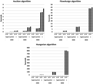
First, we give a detailed review of two algorithms that solve the minimization case of the assignment problem, the Bertsekas auction algorithm and the Goldberg & Kennedy algorithm. It was previously alluded that both algorithms are equivalent. We give a detailed proof that these algorithms are equivalent. Also, we perform experimental results comparing the performance of three algorithms for the assignment problem: the \(\epsilon \) - scaling auction algorithm , the Hungarian algorithm and the FlowAssign algorithm . The experiment shows that the auction algorithm still performs and scales better in practice than the other algorithms which are harder to implement and have better theoretical time complexity.

This is a preview of subscription content, log in via an institution to check access.

Access this article

Price includes VAT (Russian Federation)

Instant access to the full article PDF.

Rent this article via DeepDyve

Institutional subscriptions

Similar content being viewed by others

Some results on an assignment problem variant

Integer Programming

A Full Description of Polytopes Related to the Index of the Lowest Nonzero Row of an Assignment Matrix

Bertsekas, D.P.: The auction algorithm: a distributed relaxation method for the assignment problem. Annal Op. Res. 14 , 105–123 (1988)

Article   MathSciNet   Google Scholar  

Bertsekas, D.P., Castañon, D.A.: Parallel synchronous and asynchronous implementations of the auction algorithm. Parallel Comput. 17 , 707–732 (1991)

Article   Google Scholar  

Bertsekas, D.P.: Linear network optimization: algorithms and codes. MIT Press, Cambridge, MA (1991)

MATH   Google Scholar  

Bertsekas, D.P.: The auction algorithm for shortest paths. SIAM J. Optim. 1 , 425–477 (1991)

Bertsekas, D.P.: Auction algorithms for network flow problems: a tutorial introduction. Comput. Optim. Appl. 1 , 7–66 (1992)

Bertsekas, D.P., Castañon, D.A., Tsaknakis, H.: Reverse auction and the solution of inequality constrained assignment problems. SIAM J. Optim. 3 , 268–299 (1993)

Bertsekas, D.P., Eckstein, J.: Dual coordinate step methods for linear network flow problems. Math. Progr., Ser. B 42 , 203–243 (1988)

Bertsimas, D., Tsitsiklis, J.N.: Introduction to linear optimization. Athena Scientific, Belmont, MA (1997)

Google Scholar  

Burkard, R., Dell’Amico, M., Martello, S.: Assignment Problems. Revised reprint. SIAM, Philadelphia, PA (2011)

Gabow, H.N., Tarjan, R.E.: Faster scaling algorithms for network problems. SIAM J. Comput. 18 (5), 1013–1036 (1989)

Goldberg, A.V., Tarjan, R.E.: A new approach to the maximum flow problem. J. Assoc. Comput. Mach. 35 , 921–940 (1988)

Goldberg, A.V., Tarjan, R.E.: Finding minimum-cost circulations by successive approximation. Math. Op. Res. 15 , 430–466 (1990)

Goldberg, A.V., Kennedy, R.: An efficient cost scaling algorithm for the assignment problem. Math. Programm. 71 , 153–177 (1995)

MathSciNet   MATH   Google Scholar  

Goldberg, A.V., Kennedy, R.: Global price updates help. SIAM J. Discr. Math. 10 (4), 551–572 (1997)

Kuhn, H.W.: The Hungarian method for the assignment problem. Naval Res. Logist. Quart. 2 , 83–97 (1955)

Kuhn, H.W.: Variants of the Hungarian method for the assignment problem. Naval Res. Logist. Quart. 2 , 253–258 (1956)

Lawler, E.L.: Combinatorial optimization: networks and matroids, Holt. Rinehart & Winston, New York (1976)

Orlin, J.B., Ahuja, R.K.: New scaling algorithms for the assignment ad minimum mean cycle problems. Math. Programm. 54 , 41–56 (1992)

Ramshaw, L., Tarjan, R.E., Weight-Scaling Algorithm, A., for Min-Cost Imperfect Matchings in Bipartite Graphs, : IEEE 53rd Annual Symposium on Foundations of Computer Science. New Brunswick, NJ 2012 , 581–590 (2012)

Zaki, H.: A comparison of two algorithms for the assignment problem. Comput. Optim. Appl. 4 , 23–45 (1995)

Download references

Acknowledgements

This research was partially supported by SNI and CONACyT.

Author information

Authors and affiliations.

Banco de México, Mexico City, Mexico

Carlos A. Alfaro & Marcos C. Vargas

Mountain View, CA, 94043, USA

Sergio L. Perez

Departamento de Matemáticas, CINVESTAV del IPN, Apartado postal 14-740, 07000, Mexico City, Mexico

Carlos E. Valencia

You can also search for this author in PubMed   Google Scholar

Corresponding author

Correspondence to Carlos A. Alfaro .

Ethics declarations

Conflict of interest.

There is no conflict of interest.

Additional information

Publisher's note.

Springer Nature remains neutral with regard to jurisdictional claims in published maps and institutional affiliations.

The authors were partially supported by SNI and CONACyT.

Rights and permissions

Reprints and permissions

About this article

Alfaro, C.A., Perez, S.L., Valencia, C.E. et al. The assignment problem revisited. Optim Lett 16 , 1531–1548 (2022). https://doi.org/10.1007/s11590-021-01791-4

Download citation

Received : 26 March 2020

Accepted : 03 August 2021

Published : 16 August 2021

Issue Date : June 2022

DOI : https://doi.org/10.1007/s11590-021-01791-4

Share this article

Anyone you share the following link with will be able to read this content:

Sorry, a shareable link is not currently available for this article.

Provided by the Springer Nature SharedIt content-sharing initiative

• Assignment problem
• Bertsekas auction algorithm
• Combinatorial optimization and matching
• Find a journal
• Publish with us
• Track your research

• MapReduce Algorithm
• Linear Programming using Pyomo
• Networking and Professional Development for Machine Learning Careers in the USA
• Predicting Employee Churn in Python
• Airflow Operators

Solving Assignment Problem using Linear Programming in Python

Learn how to use Python PuLP to solve Assignment problems using Linear Programming.

In earlier articles, we have seen various applications of Linear programming such as transportation, transshipment problem, Cargo Loading problem, and shift-scheduling problem. Now In this tutorial, we will focus on another model that comes under the class of linear programming model known as the Assignment problem. Its objective function is similar to transportation problems. Here we minimize the objective function time or cost of manufacturing the products by allocating one job to one machine.

If we want to solve the maximization problem assignment problem then we subtract all the elements of the matrix from the highest element in the matrix or multiply the entire matrix by –1 and continue with the procedure. For solving the assignment problem, we use the Assignment technique or Hungarian method, or Flood’s technique.

The transportation problem is a special case of the linear programming model and the assignment problem is a special case of transportation problem, therefore it is also a special case of the linear programming problem.

In this tutorial, we are going to cover the following topics:

Assignment Problem

A problem that requires pairing two sets of items given a set of paired costs or profit in such a way that the total cost of the pairings is minimized or maximized. The assignment problem is a special case of linear programming.

For example, an operation manager needs to assign four jobs to four machines. The project manager needs to assign four projects to four staff members. Similarly, the marketing manager needs to assign the 4 salespersons to 4 territories. The manager’s goal is to minimize the total time or cost.

Problem Formulation

A manager has prepared a table that shows the cost of performing each of four jobs by each of four employees. The manager has stated his goal is to develop a set of job assignments that will minimize the total cost of getting all 4 jobs.  

Initialize LP Model

In this step, we will import all the classes and functions of pulp module and create a Minimization LP problem using LpProblem class.

Define Decision Variable

In this step, we will define the decision variables. In our problem, we have two variable lists: workers and jobs. Let’s create them using  LpVariable.dicts()  class.  LpVariable.dicts()  used with Python’s list comprehension.  LpVariable.dicts()  will take the following four values:

• First, prefix name of what this variable represents.
• Second is the list of all the variables.
• Third is the lower bound on this variable.
• Fourth variable is the upper bound.
• Fourth is essentially the type of data (discrete or continuous). The options for the fourth parameter are  LpContinuous  or  LpInteger .

Let’s first create a list route for the route between warehouse and project site and create the decision variables using LpVariable.dicts() the method.

Define Objective Function

In this step, we will define the minimum objective function by adding it to the LpProblem  object. lpSum(vector)is used here to define multiple linear expressions. It also used list comprehension to add multiple variables.

Define the Constraints

Here, we are adding two types of constraints: Each job can be assigned to only one employee constraint and Each employee can be assigned to only one job. We have added the 2 constraints defined in the problem by adding them to the LpProblem  object.

Solve Model

In this step, we will solve the LP problem by calling solve() method. We can print the final value by using the following for loop.

From the above results, we can infer that Worker-1 will be assigned to Job-1, Worker-2 will be assigned to job-3, Worker-3 will be assigned to Job-2, and Worker-4 will assign with job-4.

In this article, we have learned about Assignment problems, Problem Formulation, and implementation using the python PuLp library. We have solved the Assignment problem using a Linear programming problem in Python. Of course, this is just a simple case study, we can add more constraints to it and make it more complicated. You can also run other case studies on Cargo Loading problems , Staff scheduling problems . In upcoming articles, we will write more on different optimization problems such as transshipment problem, balanced diet problem. You can revise the basics of mathematical concepts in  this article  and learn about Linear Programming  in this article .

• Solving Blending Problem in Python using Gurobi
• Transshipment Problem in Python Using PuLP

You May Also Like

Naive Bayes Classification using Scikit-learn

Solving Cargo Loading Problem using Integer Programming in Python

Dimensionality Reduction using PCA

Maximisation in an Assignment Problem: Optimizing Assignments for Maximum Benefit

Table of Contents

This blog will explain how to solve assignment problems using optimization techniques to achieve maximum results. Learn the basics, step-by-step approach, and real-world applications of maximizing assignment problems.

In an assignment problem, the goal is to assign n tasks to n agents in such a way that the overall cost or benefit is minimized or maximized. The maximization problem arises when the objective is to maximize the overall benefit rather than minimize the cost.

Understanding Maximisation in an Assignment Problem

The maximization problem can be solved using the Hungarian algorithm, which is a special case of the transportation problem. The algorithm involves converting the assignment problem into a matrix, finding the minimum value in each row, and subtracting it from all the elements in that row. Similarly, we find the minimum value in each column and subtract it from all the elements in that column. This is known as matrix reduction.

Next, we cover all zeros in the matrix using the minimum number of lines. A line covers a row or column that contains a zero. If the minimum number of lines is n, an optimal solution has been found. Otherwise, we continue with the next step.

In step three, we add the minimum uncovered value to each element covered by two lines, and subtract it from each uncovered element. Then, we return to step two and repeat until an optimal solution is found.

Solving Maximisation in an Assignment Problem

The above approach provides a step-by-step process to maximize an assignment problem. Here are the steps in summary:

• Convert the assignment problem into a matrix.
• Reduce the matrix by subtracting the minimum value in each row and column.
• Cover all zeros in the matrix with the minimum number of lines.
• Add the minimum uncovered value to each element covered by two lines and subtract it from each uncovered element.
• Repeat from step two until an optimal solution is found.

Real-World Applications

Maximization in an Assignment Problem has numerous real-world applications. For example, it can be used to optimize employee allocation to projects, to allocate tasks in a manufacturing process, or to assign jobs to machines for maximum productivity. By using optimization techniques to maximize the benefits of an assignment problem, businesses can save time, money, and resources.

This blog has provided an overview of Maximisation in an Assignment Problem, explained how to solve it using the Hungarian algorithm, and discussed real-world applications. By following the step-by-step approach, you can optimize your assignments for maximum benefit.

How useful was this post?

Click on a star to rate it!

Average rating 5 / 5. Vote count: 2

No votes so far! Be the first to rate this post.

We are sorry that this post was not useful for you! 😔

Let us improve this post!

Tell us how we can improve this post?

Operations Research

1 Operations Research-An Overview

• History of O.R.
• Approach, Techniques and Tools
• Phases and Processes of O.R. Study
• Typical Applications of O.R
• Limitations of Operations Research
• Models in Operations Research
• O.R. in real world

2 Linear Programming: Formulation and Graphical Method

• General formulation of Linear Programming Problem
• Optimisation Models
• Basics of Graphic Method
• Important steps to draw graph
• Multiple, Unbounded Solution and Infeasible Problems
• Solving Linear Programming Graphically Using Computer
• Application of Linear Programming in Business and Industry

3 Linear Programming-Simplex Method

• Principle of Simplex Method
• Computational aspect of Simplex Method
• Simplex Method with several Decision Variables
• Two Phase and M-method
• Multiple Solution, Unbounded Solution and Infeasible Problem
• Sensitivity Analysis
• Dual Linear Programming Problem

4 Transportation Problem

• Basic Feasible Solution of a Transportation Problem
• Modified Distribution Method
• Stepping Stone Method
• Unbalanced Transportation Problem
• Degenerate Transportation Problem
• Transhipment Problem
• Maximisation in a Transportation Problem

5 Assignment Problem

• Solution of the Assignment Problem
• Unbalanced Assignment Problem
• Problem with some Infeasible Assignments
• Maximisation in an Assignment Problem
• Crew Assignment Problem

6 Application of Excel Solver to Solve LPP

• Building Excel model for solving LP: An Illustrative Example

7 Goal Programming

• Concepts of goal programming
• Goal programming model formulation
• Graphical method of goal programming
• The simplex method of goal programming
• Using Excel Solver to Solve Goal Programming Models
• Application areas of goal programming

8 Integer Programming

• Some Integer Programming Formulation Techniques
• Binary Representation of General Integer Variables
• Unimodularity
• Cutting Plane Method
• Branch and Bound Method
• Solver Solution

9 Dynamic Programming

• Dynamic Programming Methodology: An Example
• Definitions and Notations
• Dynamic Programming Applications

10 Non-Linear Programming

• Solution of a Non-linear Programming Problem
• Convex and Concave Functions
• Kuhn-Tucker Conditions for Constrained Optimisation
• Quadratic Programming
• Separable Programming
• NLP Models with Solver

11 Introduction to game theory and its Applications

• Important terms in Game Theory
• Saddle points
• Mixed strategies: Games without saddle points
• 2 x n games
• Exploiting an opponent’s mistakes

12 Monte Carlo Simulation

• Reasons for using simulation
• Monte Carlo simulation
• Limitations of simulation
• Steps in the simulation process
• Some practical applications of simulation
• Two typical examples of hand-computed simulation
• Computer simulation

13 Queueing Models

• Characteristics of a queueing model
• Notations and Symbols
• Statistical methods in queueing
• The M/M/I System
• The M/M/C System
• The M/Ek/I System
• Decision problems in queueing