how to link worksheet

• PRO Courses Guides New Tech Help Pro Expert Videos About wikiHow Pro Upgrade Sign In
• EXPLORE Tech Help Pro About Us Random Article Quizzes Request a New Article Community Dashboard This Or That Game Popular Categories Arts and Entertainment Artwork Books Movies Computers and Electronics Computers Phone Skills Technology Hacks Health Men's Health Mental Health Women's Health Relationships Dating Love Relationship Issues Hobbies and Crafts Crafts Drawing Games Education & Communication Communication Skills Personal Development Studying Personal Care and Style Fashion Hair Care Personal Hygiene Youth Personal Care School Stuff Dating All Categories Arts and Entertainment Finance and Business Home and Garden Relationship Quizzes Cars & Other Vehicles Food and Entertaining Personal Care and Style Sports and Fitness Computers and Electronics Health Pets and Animals Travel Education & Communication Hobbies and Crafts Philosophy and Religion Work World Family Life Holidays and Traditions Relationships Youth
• Browse Articles
• Learn Something New
• Quizzes Hot
• This Or That Game
• Train Your Brain
• Explore More
• Support wikiHow
• About wikiHow
• Log in / Sign up
• Computers and Electronics
• Spreadsheets
• Microsoft Excel

How to Link Sheets in Excel

Last Updated: April 3, 2024 Fact Checked

This article was co-authored by wikiHow Staff . Our trained team of editors and researchers validate articles for accuracy and comprehensiveness. wikiHow's Content Management Team carefully monitors the work from our editorial staff to ensure that each article is backed by trusted research and meets our high quality standards. This article has been fact-checked, ensuring the accuracy of any cited facts and confirming the authority of its sources. This article has been viewed 434,091 times. Learn more...

This wikiHow teaches you how to link data between multiple worksheets in a Microsoft Excel workbook. Linking will dynamically pull data from a sheet into another, and update the data in your destination sheet whenever you change the contents of a cell in your source sheet. [1] X Trustworthy Source Microsoft Support Technical support and product information from Microsoft. Go to source

Quick Guide for Linking Sheets in Excel

Click an empty cell in your destination sheet, then type an equal sign (=) and click on the source sheet, then the source cell in the source sheet, and hit Enter. Check to make sure that the destination cell's formula has been altered.

• Alternatively, you can manually write this formula in the formula bar. It should look like =<SheetName>! , where "<SheetName>" is replaced with the name of your source sheet. [5] X Trustworthy Source Microsoft Support Technical support and product information from Microsoft. Go to source

• For example, if you're pulling data from cell D12 in Sheet1, the formula should look like =Sheet1!D12 . [7] X Trustworthy Source Microsoft Support Technical support and product information from Microsoft. Go to source

• You can drag and expand the range of linked cells in any direction. This could include the entire worksheet, or only parts of it.

Community Q&A

You Might Also Like

• ↑ https://support.microsoft.com/en-us/office/update-workbook-links-21e995b5-bab1-4328-8ab3-dd357fe0e653
• ↑ https://support.microsoft.com/en-gb/office/work-with-links-in-excel-7fc80d8d-68f9-482f-ab01-584c44d72b3e
• ↑ https://support.microsoft.com/en-us/office/create-workbook-links-c98d1803-dd75-4668-ac6a-d7cca2a9b95f
• ↑ https://support.microsoft.com/en-us/office/create-or-change-a-cell-reference-c7b8b95d-c594-4488-947e-c835903cebaa

About This Article

1. Open Excel. 2. Click your destination cell. 3. Type " = ". 4. Click another sheet. 5. Click your source cell. 6. Press Enter on your keyboard. Did this summary help you? Yes No

• Send fan mail to authors

Is this article up to date?

Featured Articles

Trending Articles

Watch Articles

• Terms of Use
• Privacy Policy
• Do Not Sell or Share My Info
• Not Selling Info

wikiHow Tech Help Pro:

Level up your tech skills and stay ahead of the curve

Home   »   Excel Basics

How to Link Data Between Excel Worksheets

November 24, 2023   -   BY Pat Kearns

Microsoft Excel provides the ability for cells in one worksheet to be linked to cells in other worksheets in the same or different workbook.

In this tutorial, you'll learn how to link worksheet data in all versions of Excel. It's easy, and we'll show you several different ways to do it!

A KeynoteSupport.com Tutorial

Table of Contents

Why link worksheet data, how linking spreadsheet data works, formula for linking worksheet cells, how to create a worksheet link, how to link a range of cells, linking to worksheets in different workbooks, moving worksheets with external cell references, handling linked data security warning messages.

Though we provide links to each section of this tutorial, we recommend it be read from start to finish.

Creating links between worksheets can be a huge productivity boost. Using external cell references in a worksheet can cut down on entering the same data in multiple worksheets.

For example, a Sales Manager can have a detailed sheet for each sales representative, and a summary sheet to compare team performance. Prices can be stored in a master sheet to which other worksheets link.

Creating links between multiple sheets greatly helps with data integrity. If prices are kept in one worksheet and others link to it, there is much less chance of data entry errors.

In addition, multiple Excel users aren't having to enter the same data, so it saves time and increases employee productivity.

First we'll show you exactly how linking works, then we'll show you, step-by-step, how to link worksheet data. You'll be a pro in no time!

When we link data, we tell Excel to display data from another worksheet. The worksheet that has the data that we want copied to our worksheet is called the source worksheet .

The worksheet that we're currently working in that wants the data is called the destination worksheet .

And the method in which we tell Excel to go to another worksheet and get the data is called a link formula . We show you three different ways of creating link formulas.

The link formula syntax is =SheetName ! CellReference where SheetName is the name of the source worksheet, and CellReference is the cell from the source worksheet that contains the data.

In the example below, we entered =Toronto!B6 in the destination sheet to display the units sold from the source worksheet Toronto. Study the image below of the two spreadsheets.

These two worksheets are in the same Excel workbook. We can see the worksheet names, Toronto and Summary, on the tabs at the bottom of the worksheet. Worksheet names can be edited .

Any time the data from the source worksheet changes, the destination worksheet will show the new data the next time it is opened.

We'll look at three methods for creating a link formula . These instructions assume that the source and destination worksheets are in the same workbook. If not, go to Linking to Worksheets in Different Workbooks below.

Also, make sure that you always format the cell that will contain the link formula before entering the formula.

✦ Link Worksheet Data - Method One ✦

In some ways, we prefer the manual way of entering the link formula we discussed above (Method 3) because we don't like to jump from worksheet to worksheet. But try each method to see which one you like the best.

This method begins in the destination worksheet. Format the cell that will contain the link formula, and keeping the mouse cursor in that cell, follow the directions below.

• In the destination worksheet, with the cursor in the cell that will contain the link formula, type an equal sign but don't press the Enter key (figure 1).
• Jump to the source worksheet, click in the cell with the data to be linked (figure 2) and press Enter.

If done correctly, Excel returns to the destination sheet and displays the linked data.

✦ Link Worksheet Data - Method Two ✦

With Method Two, we begin in the source and end in the destination sheet. We'll copy from the cell in the source worksheet and Paste Link in the destination sheet. Follow these steps.

• Format the cell in the destination worksheet that will contain the link formula.
• Go to the source worksheet and copy * the data to be linked. Like the example in Method One, we're bringing the value of cell B6 from the Paris sheet into our summary worksheet.
• In the destination sheet, click the cell where you want the link formula. Then, on the Home tab of the ribbon, click the Paste icon (Clipboard group) and click Paste Link under Paste Options (see figure 3). (Old versions of Excel: Edit ⇒ Paste Special ⇒ Paste Link)
• Return to the source worksheet and press ESC key to remove the animated border on the source cell.

The cell in the destination worksheet that contains the formula will show the copied and linked data, and the link formula displays in the formula bar (figure 4).

With these first two methods, Excel creates the formula =Paris!$B$6 and wraps the source cell with dollar signs ( absolute cell reference ).

* Copy methods: 1) keyboard shortcut Ctrl + C ,   2) right-click menu,   3) copy button on the ribbon's Home tab.

✦ Manually Write Formulas - Method 3 ✦

Entering formulas manually is not difficult ... see Link Formula Syntax above. Without any spaces in between, type equal sign, sheet name, exclamation mark, cell reference : =SheetName ! CellReference .

If you have complex or multiple formulas to enter, open a Notepad file, create the formulas, copy and paste them into the destination cell, and modify as needed.

Don't worry about capitalizing worksheet names. If the first letter of the worksheet name is capitalized and you enter the name in the formula without the capital letter, Excel will add it. And vice versa. See Naming and Renaming Worksheets .

In linking formulas, spaces or special characters must be wrapped in single quotes . If the worksheet name is Retail Prices , then a linking formula, manually created or generated by Excel, look like the following:   ='Retail Prices'!B6 . Therefore, life is easier if worksheet names, on the tabs at the bottom of the workbook, are one word long.

Because of internal workings, Excel will automatically wraps worksheet names C or R in single quotes.

To link a range of cells, select the cells and click Copy. In the destination sheet, click the cell where the upper-left cell of the range should be located and click Paste ⇒ Paste Link on the Home tab.

Cell values in the range will be linked, and will display on the destination sheet. Each cell in the range will contain its own link formula which references the corresponding cell in the source worksheet.

If the worksheets are in different workbooks in the same folder or directory , the formula must also include the workbook name in brackets as shown.

=[BookName.xlsx]SheetName!CellReference

=[BookName.xlsx]SheetName! CellReference

If the workbooks are in different folders, the formula would have to include the complete file path as well, so it is best to avoid this situation. Don't forget that versions older than Excel 2007 have a file extension of xls .

If the source and destination worksheets are in the same workbook, moving the workbook to a different folder or even a different computer should not be a problem.

However, if one of the worksheets is moved to a different workbook, the link will break. If the worksheets are in different workbooks and one or both are moved, results are unpredictable.

Companies that store shared worksheets on network servers have additional factors to consider that are outside the scope of this tutorial.

The next time you open the destination worksheet, you will undoubtedly see one of the following security alerts, warning you that Automatic update of links has been disabled .

Procedures for responding to this message and a subsequent security warning differ depending on your version of Excel.

For detailed information and the procedure for permanently disabling these security warnings, please see Automatic Updates When Linking Data and Charts .

Linking worksheet data in Excel is a great feature to know and use. Try the three different methods and choose the one that works best for you.

Related Tutorials

• How to Sum Data in the Same Cell Address from Multiple Sheets
• How to Sum from Different Cell Addresses Across Multiple Sheets
• Automatic Updates When Linking Data and Charts in Excel

• Ablebits blog

How to add a hyperlink to another worksheet

In this article I'll show you 3 ways how you can add hyperlinks into your Excel workbook to easily navigate between numerous worksheets. You'll also learn how to change a link destination and modify its format. If you don't need a hyperlink any more, you'll see how to quickly remove it.

If you are a real Internet surfer, you know firsthand about the bright sides of hyperlinks. Clicking on hyperlinks you instantly get access to other information no matter where it is located. But do you know the benefits of spreadsheet hyperlinks in Excel workbooks? The time has come to discover them and start using this great Excel feature.

One of the ways you can put spreadsheet hyperlinks to good use is to create a table of contents of your workbook. Excel internal hyperlinks will help you to quickly jump to the necessary part of the workbook without hunting through multiple worksheets.

Insert a hyperlink in Excel

If you need to add a hyperlink in Excel 2016 or 2013, you can choose one of the following hyperlink types: a link to an existing or new file, to a web page or e-mail address. Since the subject of this article is creating a hyperlink to another worksheet in the same workbook, below you'll find out three ways to do that.

Add a hyperlink from the context menu

The first method of creating a hyperlink within one workbook is to use the Hyperlink command .

• Select a cell where you want to insert a hyperlink.

• Choose Place in This Document in the Link to section if your task is to link the cell to a specific location in the same workbook.
• Select the worksheet that you want to link to in the Or select a place in this document field.
• Enter the cell address in the Type the cell reference box if you want to link to a certain cell of another worksheet.

Excel HYPERLINK function

Excel has a HYPERLINK function that you can also use for creating links between spreadsheets in the workbook . If you are not good at entering Excel formulas immediately in the Formula bar, do the following:

• Select the cell to which you want to add a hyperlink.
• Go to Function Library on the FORMULAS tab.

Note. It's not a must to enter friendly_name. But if you want the hyperlink to look neat and clear, I'd recommend to do it. If you don't type in friendly_name, the cell will display the link_location as the jump text.

Tip. If you don't know what address to enter, just use the Select range icon to pick the destination cell.

Note. It is crucial to type the number sign. It indicates that the location is within the current workbook. If you forget to enter it, the link won't work and an error will appear when you click on it.

• Enter Friendly_name that you want to display in the cell.

Insert a link by cell drag-and-drop

The quickest way of creating hyperlinks within one workbook is using the drag-and-drop technique . Let me show you how it works.

As an example, I'll take a workbook of two sheets and create a hyperlink in Sheet 1 to a cell in Sheet 2.

Note. Make sure that the workbook is saved because this method doesn't work in new workbooks.

• Select the hyperlink destination cell in Sheet 2.

• Press the Alt key and mouse over the Sheet 1 tab. Having the Alt key pressed automatically takes you to the other sheet. Once Sheet 1 is activated, you can stop holding the key.

• Release the right mouse button for the popup menu to appear.

After you do that, the hyperlink appears in the cell. When you click on it, you'll switch to the destination cell in Sheet 2.

Edit a hyperlink

You can edit an existing hyperlink in your workbook by changing its destination, its appearance, or the text that is used to represent it.

Change link destination

As this article deals with hyperlinks between spreadsheets of the same workbook, the hyperlink destination in this case is a specific cell from another spreadsheet. If you want to change the hyperlink destination, you need to modify the cell reference or choose another sheet. You can do both, if necessary.

• Right-click the hyperlink you want to edit.

Note. There are, at least, two more ways to open the Edit Hyperlink dialog. You can press Ctrl + K or click on Hyperlink in the Links group on the INSERT tab. But don't forget to select the necessary cell before doing it.

• Update the information in the appropriate fields of the Edit Hyperlink dialog.

Note. In case you used Method 2 to add a hyperlink in Excel, you need to edit the formula to change the hyperlink destination. Select the cell that contains the link, and then place the cursor in the Formula bar to edit it.

Modify hyperlink format

Most of the time hyperlinks are shown as an underlined text of blue color. If the typical appearance of hyperlink text seems to you boring and you'd like to stand out of the crowd, go ahead and read below how to do it:

• Go to the Styles group on the HOME tab.
• Open the Cell Styles list.
• Right-click on Hyperlink to change the appearance of the hyperlink that was not clicked. Or right-click Followed Hyperlink if the hyperlink was activated.

• Click on Format in the Styles dialog box.
• Make the necessary changes in the Format Cells dialog window. Here you can change the hyperlink alignment and font or add fill color.
• When you are done, click OK.
• Make sure that all the changes are marked under Style includes in the Style dialog box.

Remove a hyperlink

It will take you a few seconds and no efforts to delete a hyperlink from the worksheet.

• Right-click the hyperlink you want to remove.

The text remains in the cell, but it is no longer a hyperlink.

Note. If you want to delete a hyperlink and the text that represents it, right-click the cell that contains the link and choose the Clear Contents option from the menu.

This trick helps you to delete a single hyperlink. If you want to know how to remove multiple (all) hyperlinks from Excel worksheets at a time , follow the link to our previous blog post.

You may also be interested in

• How to use Excel Hyperlink function to create different link types.
• Excel Hyperlink: how to create, change and remove
• How to quickly extract domain names from URLs in Excel.
• How to recover unsaved Excel file or restore its previous version
• How to find and fix broken links in Excel
• How to find and remove external links in Excel
• How to make hyperlinks work in Outlook

Table of contents

127 comments

We have spreadsheet with close to 40 tabs. Teh names of those tabs are in column A. I would like to use that column A reference to create the hyperlink based on the value in column A. Is this possible?

Hi! If I understand you correctly, you can use the HYPERLINK function to create a hyperlink based on a cell value. Try to follow the recommendations from this article: How to use Excel HYPERLINK function to create different link types

how to link a cell from one sheet to all other sheets in the same workbook ? For Example on Sheet 1 in Cell A1 and A2 I have data, the same data should flow on rest all of the sheets in the workbook. Do we have any formulas ?

An Excel formula cannot transfer data to another cell. It can get data from another cell. So on each worksheet, write a formula that will get data from that cell A1. It will be a regular Excel cell reference. Read more: Excel reference to another sheet or workbook (external reference) . You can transfer data to other cells on other worksheets using a VBA macro.

Hi, I have a query.

I have a summary sheet (Summary) and four different assessment templates as different sheets (SheetA, SheetB, SheetC, SheetD)

In summary sheet there will be a formula in Column D of each row (D3, D4, D5, D6, D7....D50) which Assessment sheet to be used.

Based on the inputs in Column A, B, C, value will appear in Column D as " Use Sheet B" or "Use Sheet D" or "Use Sheet A".

Now how to link the result in Column D of summary sheet into respective Assessment sheets?

Please help on this.

Hi! You can create a dynamic reference using the INDIRECT function. The following tutorial should help: INDIRECT formula to dynamically refer to another worksheet .

I want to make a hyperlink to a specific cell , and even if the sheet and the rows and the lines are modified and this exact cell is moved, the hyperlink should be moved with the cell, and not stay consistent to the prior selection , is this possible?

Hi! Unfortunately, Excel hyperlinks do not automatically change when a workbook is modified.

You can name your cell, here I used "MyCell" and then use the following syntax : =HYPERLINK("#MyCell","Label")

does not seem to relate to 365 - the bookmark option is not even available. Such a helpful, useful tool just eradicated from simple usage

i want to link cell to cell in same sheet can you help me. example i want to click one cell and cell go to another cell linked with other.

Hi! Here is the article that may be helpful to you: Hyperlink in Excel: how to create, edit and remove .

I want a hyperlink to send me to another sheet which then will linkbyo a drop down list that will match the name on the oth page.. is this possible?

Hi! If I understand correctly, you can hyperlink to a cell with a drop-down list. Read more here: Hyperlink in Excel: how to create, edit and remove .

Hi I have 2 excel sheets. I want to link data tab-wise. In the main excel sheet data are city wise and in another excel sheet I have data on each tab city wise

I want to link those excel 1 with excel 2 tabs

can we do this

Hi! Unfortunately, I can't see your data and I don't really understand what you want to link. Ask a specific question about the formula and I'll try to help.

I want to create link/objective in excel for each row. so that other can attach the receipts. is there any other way to do this other than hyperlink..

Thank you, Thayappa

I want to create a hyperlink which contains a jump to another sheet in the same workbook. The name of the sheet shall not be "hard coded" but taken from a cell. For illustration:

- cell B4 contains "Sheet14", which is the name of a sheet - desired hyperlink: =hyperlink (...B4...!A1;"Jump to sheet")

Hello! I believe the following formula will help you solve your task:

=HYPERLINK("#"&B4&"!A1","Jump to sheet")

Great, this works - thank you!

Can any one help I have two sheets A and B Sheet A is for user Sheet B for email

I have hyperlink "mailto:" on sheetB Cell B6 and I have hide this sheet , now on SheetA Cell A2 I want to create link with hided sheet's cell B6 whenever I click on A2 it work like I clicked on B6 . How can I link with A2 to B6

Hello! If I understood your question correctly, create a external reference to a cell in another worksheet, and then you can hide that sheet. You can also just write a link to a cell using the F2 key to edit it.

Hello, I have an Excel workbook with several sheets in it - the first sheet is a summary sheet listing each employee, and then every employee has an individual sheet. I have set up hyperlinks between the each worksheet and the summary sheet for easy navigation backwards and forwards. However, when I add a new employee row in the summary sheet, the hyperlinks do not update on the individual employee sheets, therefore when I now click on 'Joe Bloggs'' hyperlink, to return to the summary sheet, it brings me to the row above/below that reference. So my question is, is there anyway to make dynamic hyperlinks which would update when a new row is added into that first summary sheet? Thanks for your help, all advice appreciated.

Hello! You can create dynamic hyperlinks using the MATCH function . The formula for a dynamic hyperlink could look like this:

=HYPERLINK("#"&"SummarySheet!B"&(MATCH(B2, SummarySheet!$B$3:$B$100,0)+2),"Click Here to See Data")

where: B2 - employee name The # sigh indicates the formula to refer to the same workbook. SummarySheet!B - is a reference to the sheet name and column name in the symmary table. MATCH(B2, SummarySheet!$B$3:$B$100,0) returns the position of the corresponding employee in the summary sheet. 2 is added to it because the data list starts on the third row. I hope my advice will help you solve your task.

Thanks so much Alexander. I have entered the following formula: =HYPERLINK("#"&"EE''s!''&(MATCH(B10,EE''s'!$B$6:$B$500,0)+6),""Click Here to See Data") My Employee's worksheet is named EE's and the Employee Name is in cell B10. The list of names start in cell B6. When I click on hyperlink, I'm getting an error message to say that the reference isn't valid. Have I missed something?

Thanks for your help, I appreciate it. Dawn

Hi! If the worksheet name includes spaces or non-alphabetical characters, you must enclose it in single quotation marks. For more information, please visit: How to reference another sheet in Excel .

Hello, Can someone please help me on this. I have 2 documents, A and B. Document A is the master sheet. Document B has the following sheets p&L 1st qarter, p&l 2nd quarter etc. How can i create a hyperlink on my mastersheet (Docment A) that when clicked it will specifically open p&l 2nd quarter sheet on Document B?

Hi! Have you tried the ways described in this blog post?

I tried every thing available online on HYPERLINK function to enter a syntax that enables to have a DYNAMIC excel worksheet name, so that I could paste this worksheet anywhere and it will pick 1) automatically the worksheet name and execute HYPERLINK ii) if a recipient of this Excel file changes the name of the current worksheet -it will still open the Hyperlink with the new worksheet name. So far I was not successful Having read your help on Hyperlinks I know your solution will work - Thanks so much Shall make another post of the success kanil

have you got solution to this your hyperlink problem I'm interested pls kindly assist

i want to know how to do hyperlink fixed ...for example.. i use the hyperlink for column B5 and B7 title after that i need to add column on B5 some data under B5 title hyperlink for B7 show error...i need to hyperlink it again for B7 column that move down to B19

Is there a way to click a cell/hyperlink on sheet 1 which takes you to a filtered list on sheet 2 within the same workbook.

Ive seen people writing code o do this but its beyond my skill level.

Hello! Perhaps this instruction will be useful to you: Hyperlink to a sheet or cell in the current workbook .

I wantt to know how I can link a cell in sheet 1 to sheet 2. But if I change the name of the sheet 2 to something different, the link would remain intact.

Hi! I hope you have studied the recommendations in the tutorial above. It contains answers to your question.

I am having an issue that I was hopping someone here can maybe answer or have a solution to. I use the hyperlink function to reference a specific cell within the same workbook, but on a different sheet or page (Sheet A). When on Sheet B & I click on the hyperlink that takes me exactly to the correct & corresponding cell on Sheet A.

But then, when on sheet A, I will sort the data to fit my needs at any given time. The rub/ issue I am experiencing is that once I sort on Sheet A the hyperlink on Sheet B will now link to the old location and not update.

Example: On sheet B I click on hyperlink. Excel jumps over to Sheet A, Cell A4. On Sheet A I then sort the data in a column from ascending order to descending. The data on Sheet A updates and moves around accordingly. Then when I go back to Sheet B, and click on the same hyperlink as before, I am redirected to Sheet A, Cell A4. However, because of the sort function & data movement, the information is now inaccurate as the hyperlink in Sheet B is still refencing the old/ previous location (Sheet A, Cell A4) when instead it should direct me to the new location (lets just say... Sheet A, Cell A1) after the sort function has completed.

Is there a way to embed a hyperlink that points to a different page & cell within the same workbook, that also updates if the "Sort & Filter" function is performed?

Thanks! Fingers Crossed!

Hello! I'm really sorry, we cannot help you with this.

in column A i have the heading ITEM, column B the heading COST and in column C the heading PROFIT. in column G (in the same sheet) i just want to type the ITEM and it must display the ITEM and the COST and the PROFIT. is it possible for you to HELP PLEASE?(each heading must display in its own cell)

Hello! Please have a look at this article: Vlookup to return multiple matches in rows . I hope my advice will help you solve your task.

I am certain I am not the only person with this question, so hopefully it can be answered easily?

I have varying reports that are compared at different intervals but all cross-reference each other. i.e., budget projections reports v actuals, receivables v outstanding etc.

So when a comparison needs to be set up, can spreadsheet cells across varying workbooks/documents be hyperlinked into one spreadsheet/workbook to produce 'differences/results' reporting?

Hope that's a clear question!? I apologize if its confusing - but I've been out of work 20 years and I'm trying to refresh all my OLD accounting skills used in much earlier versions of the software!

Hello! External references are used to link spreadsheet cells in different workbooks. I also recommend paying attention to pivot tables .

in google sheet, you can get a link to a specific row of cells. is there a similar function in excel? an example would be that I want to reference a specific row of data from an excel doc into another document like a word file.

Hello! I hope you have studied the recommendations in the tutorial above. It contains answers to your question. All links that are possible are described with the article above. A link to a Word document is also possible. You can learn more about hyperlink in Excel in this article on our blog.

Is there anyway to open hyperlink function cell , without using mouse click.

Thanks for your example to make sure to use the "#" before a cell sheet reference!

Easy guide to understand, Thanks a lot, It worked for me !

Very helpful post, thanks!

Very helpful post, thanks.

Hello Please explain how to hyperlink a complete worksheet of the same file. Or how to hyperlink sheet 1 & sheet 2. Please guide

I have a data in one excel file in which for specific part no. i had different geometrical parameters like diam., length. Now i have another excel file in which i have to prepare inspection report so, is their any way if i put the specific part no. in inspection report so all geometrical parameters will come automatically in inspection report. plz revert.

very useful post thanks

Can we use this hyperlink with data filter option?

How we know that what items are link and what are nt link in trial balance and balane sheet

Thank you :) , it's very useful .

I did not find the solution of my problem here, i need your help in this regard. i want to open sheets( also hidden sheet if possible) from the drop down menu of hyperlinks with single click without VBA. Thanks

Hello This is good one. Is there formula when you press on the link and it jumps to another sheet and finds the specific text (or part of the text)?

Thanks in advance

Hii I hyperlinked cells in a column to different location in another sheet. I added another column in the 2nd sheet and now I want to include that column to be hyperlinked too. So is it a way that that I do it once for all cells?

Very helpful. I've learned a lot from this article.

Really helpful. Thanks a lot!

Very helpful, thanks!

Good Thank You Ite Really Help full

Very useful and easy. Thank you.

Great article! Very comprehensive, informative and well set out. It is an A-Z of Hyperlinks. Thanks, it helped me greatly.

hello someone their to help me?

how to display the details in same sheet in excel? like for example sheet1: in column A1 (A1 144 and A2 145)when i click A1 144 or A2 145, the details will be display in D1 or etc. Same sheet..

I am having an issue when adding the same hyperlink from one tab to another tab only after giving the original hyperlink a friendly name. The # and "" don't seem to help. Is there a solution to this issue? For now I have just changed it to two cells, one with the hyperlink and one with the name I want to use throughout the workbook. This works, but isn't very pretty.

Please can you attach a sample file.

It makes learning faster

Can I link one spreadsheet to another so when I input the date on the first spreadsheet it will automatically populates into the other?

Its very informative, great job guys.

Hi, I had split the single sheet to multiple sheet in excel and I tried to put hyperlink am not able to get the exact cell since there are multiple cell reference in one sheet.

Thank you so much! It is very useful!

Post a comment

Excel Tutorial: How To Link Excel Worksheets

Introduction.

Linking Excel worksheets is an essential skill for anyone working with data in Excel. It allows you to create connections between different worksheets, enabling you to streamline processes, improve data accuracy, and save time. In this tutorial, we will cover the basics of how to link Excel worksheets, including the different methods and best practices to follow.

Main Points to be Covered:

• Importance of linking Excel worksheets
• Different methods for linking worksheets
• Best practices for linking worksheets

Key Takeaways

• Linking Excel worksheets is essential for streamlining processes, improving data accuracy, and saving time
• There are different methods for linking worksheets, including cell references and hyperlinks
• Best practices for linking worksheets include maintaining and updating linked worksheets, and avoiding potential challenges
• Cell references are useful for connecting data between worksheets, while hyperlinks are advantageous for navigating between worksheets
• Start implementing links in your Excel worksheets to optimize your data management and analysis

Understanding Excel Links

A. Define what it means to link Excel worksheets

Linking Excel worksheets involves creating a connection between two or more worksheets in a workbook. This allows users to reference data from one worksheet to another, making it easier to organize and analyze related information.

B. Explain the benefits of using links between worksheets

• Efficiency: Linking worksheets can help streamline data management by reducing the need to duplicate information across multiple sheets.
• Accuracy: By linking worksheets, users can ensure that any changes made to the source data are automatically updated in the linked worksheets, minimizing the risk of errors.
• Organization: Links enable users to create dynamic relationships between different sets of data, making it easier to analyze and compare information.
• Flexibility: With linked worksheets, users have the flexibility to create complex data models and reports that draw from multiple sources, providing a comprehensive view of the data.

Types of Excel Links

When it comes to linking worksheets in Excel, there are different types of links that you can use to connect data between multiple sheets. Each type of link has its own specific use and purpose. In this tutorial, we will discuss the different types of links and when to use each type.

One of the most common types of links in Excel is cell references. This type of link allows you to reference a cell or range of cells in a different worksheet or workbook. Cell references are useful for linking data between sheets and performing calculations or data analysis across multiple worksheets.

When to use cell references:

• When you need to pull data from one sheet to another for analysis or reporting
• When you want to create formulas that reference data from multiple sheets
• When you want to consolidate data from different sheets into a summary sheet

Hyperlinks are another type of link that can be used in Excel to connect worksheets. Unlike cell references, hyperlinks are clickable links that can direct the user to a different location within the same workbook, a different workbook, or even to a website or external file.

When to use hyperlinks:

• When you want to create a navigation system within your workbook for easy access to different sheets or sections
• When you want to link to external sources or websites for additional information or references
• When you want to create a clickable index or table of contents for your workbook

By understanding the different types of links in Excel and knowing when to use each type, you can effectively organize and connect your worksheets to create a more seamless and efficient workbook.

How to Create Cell References

Creating cell references in Excel allows you to link data from one worksheet to another, making it easier to organize and analyze large sets of data. Follow the steps below to create cell references in Excel:

• Select the cell: Start by selecting the cell where you want to create the cell reference.
• Enter the equal sign: Begin the cell reference with an equal sign (=) in the selected cell.
• Navigate to the target cell: Click on the worksheet tab and navigate to the cell you want to reference.
• Click Enter: After selecting the target cell, press Enter to complete the cell reference.

Examples of when cell references are useful

Cell references are useful in various scenarios, including:

• Summing data: When you need to add up values from different worksheets, cell references allow you to easily create a sum formula that automatically updates as the data changes.
• Comparing data: Cell references enable you to compare values across different worksheets, making it easier to identify trends and discrepancies.
• Creating dynamic reports: By linking data from multiple worksheets using cell references, you can create dynamic reports that update in real-time as new data is added.

Using Hyperlinks to Link Worksheets

When working on a complex Excel workbook, it can be helpful to create hyperlinks between different worksheets for easy navigation and reference. This can save time and improve the overall user experience.

A. Explain how to create hyperlinks between worksheets

• Select the cell: First, select the cell in which you want to insert the hyperlink.
• Insert Hyperlink: Then, go to the 'Insert' tab and click on 'Hyperlink'.
• Choose Location: In the dialog box that appears, select 'Place in This Document' on the left-hand side. This will allow you to select the worksheet to which you want to link.
• Select Worksheet: Finally, choose the specific worksheet and cell reference to which you want to link, and click 'OK'.

B. Discuss the advantages of using hyperlinks

There are several advantages to using hyperlinks to link worksheets in Excel. Some of these include:

• Easy Navigation: Hyperlinks make it easy to navigate between different worksheets within a workbook, especially in larger and more complex workbooks.
• Improved User Experience: By creating hyperlinks, you can improve the overall user experience and make it more intuitive for others to navigate through the workbook.
• Time-Saving: Hyperlinks can save time by allowing users to quickly jump to the relevant worksheet without having to search for it manually.
• Visual Organization: Hyperlinks can help visually organize the workbook and create a more seamless flow of information between different sections.

Best Practices for Linking Worksheets

Linking worksheets in Excel can be a powerful tool for consolidating data and creating dynamic reports. However, it's important to follow best practices to ensure the linked worksheets are easy to maintain and update.

• Use named ranges: When linking worksheets, it's a good practice to use named ranges instead of cell references. This makes it easier to update the links if the structure of the worksheets changes.
• Document the links: Keep a record of the links you create, including the source and destination of the links. This can be helpful when updating the links or troubleshooting issues.
• Update links with caution: Before updating links, ensure that the source data is available and up-to-date. Updating links with incorrect or missing data can lead to errors in the linked worksheets.
• Regularly review and update links: Periodically review the linked worksheets to ensure that the links are still valid and functioning correctly. Update any outdated links as necessary.
• Broken links: One of the common challenges when linking worksheets is broken links, especially if the source file is moved or renamed. To avoid this, use relative references instead of absolute references when creating links.
• Performance issues: Linking too many worksheets or using complex formulas can impact the performance of the workbook. To avoid this, consider simplifying the formulas or breaking the links into smaller, more manageable parts.
• Data integrity: When linking worksheets, it's important to ensure the integrity of the data. Avoid linking large amounts of data across multiple worksheets, as this can make it difficult to track changes and maintain data integrity.
• Security risks: Linked worksheets can pose security risks, especially if the source data contains sensitive information. Ensure that the source data is protected and that only authorized users have access to the linked worksheets.

In conclusion, this Excel tutorial has covered the key points of how to link Excel worksheets effectively. We discussed the benefits of linking worksheets, the steps on how to create links using formulas, and the various methods of linking data between worksheets. Now that you have learned the fundamentals of linking worksheets, I encourage you to start implementing links in your own Excel worksheets. By doing so, you can improve the efficiency and organization of your data, saving time and effort in the process.

Immediate Download

MAC & PC Compatible

Free Email Support

Related aticles

The Benefits of Excel Dashboards for Data Analysts

Unlock the Power of Real-Time Data Visualization with Excel Dashboards

Unlocking the Potential of Excel's Data Dashboard

Unleashing the Benefits of a Dashboard with Maximum Impact in Excel

Exploring Data Easily and Securely: Essential Features for Excel Dashboards

Unlock the Benefits of Real-Time Dashboard Updates in Excel

Unleashing the Power of Excel Dashboards

Understanding the Benefits and Challenges of Excel Dashboard Design and Development

Leverage Your Data with Excel Dashboards

Crafting the Perfect Dashboard for Excel

An Introduction to Excel Dashboards

How to Create an Effective Excel Dashboard

• Choosing a selection results in a full page refresh.

How to Link Cells in Excel (Same Worksheet, Between Worksheets/Workbooks)

Linked cells in Excel refer to the contents of other cells. The other cells may be in the same worksheet, other worksheets in the same workbook, or worksheets in other workbooks. 

This tutorial shows you how to link cells in Excel in the same worksheet , in different worksheets, and in different workbooks.

Table of Contents

Benefits of Linking Cells in Excel

The benefits of linking cells in Excel include:

• Data entry errors are minimized in that you do not have to re-enter the values in the referenced cells. 
• Data inconsistency is minimized. When the data in the source worksheets are changed, the values in the destination worksheets also change accordingly. 
• Workbooks are faster to open, calculate and save. When large workbooks are split into linked interdependent workbooks, you can work on the smaller workbooks one at a time without having to open all their related worksheets.    

How to Link Cells in the Same Worksheet

Let’s have a look at some methods to link cells in the same worksheet.

How to link a single cell manually

If we want to link a single cell in the same worksheet, the manual method is much faster.

In this method, we type the cell reference of the source data in the dependent cell.   

Suppose we have the following dataset of a family’s monthly cash flow in an Excel worksheet. 

We want to link cell C4 , which will contain the opening balance of cash on hand in February to cell B26 which contains the closing balance of the cash on hand in January. 

We follow the steps below:

• Select cell C4 and type in the following formula:

• Press Enter on the keyboard or click Enter on the formula bar.

Cell C4 is now linked to cell B26 and the value in cell B26 is displayed in cell C4.

If the value in cell B26 changes, the value in cell C4 will also change accordingly.

How to link a range of cells using the Paste Special feature

Using the manual method to link a range of cells is inefficient. Using the Paste Special feature in Excel is the efficient way. 

Suppose we have the following dataset.

We want to link the range E11:E24 in another location of the worksheet to the range A11:B24 which contains the expenses data. 

We proceed as follows:

• Select range A11:B24 and press Ctrl + C to copy it.

• Select cell E11.

• Open the Paste Special dialog box using any of the following techniques:

Press Ctrl + Alt + V .

In the Home tab, select the Paste Special option in the Clipboard group:

• Click the Paste Link button in the bottom left corner of the Paste Special dialog box.

The range E11:F24 is now linked to the range A11:B24. The values in range A11:B24 are now displayed in the range E11:B24. If the values in the source range change, the values in the destination range also change accordingly.

Link Cells Between Worksheets in the Same Workbook

Let’s now look at some ways you link cells in different worksheets that are in the same Excel workbook.

How to link a single cell using the point-and-click technique

Using the manual method to link cells between worksheets is not recommended because it is slow and error-prone.

The point-and-click technique is fast and accurate. It involves placing the mouse pointer on the source cell, clicking it, and pressing Enter to create the link

Suppose we have the following workbook that has three worksheets. 

The South Region and East Region worksheets contain sales data. The Summary worksheet will contain a summary of the total sales of the two regions. 

We want to link the two destination cells in the Summary worksheet shown below to the source cells in the South Region and East Region worksheets:

We use the steps below:

• Select cell B2 in the Summary worksheet and type in the equal sign (=).

• Open the South Region worksheet by clicking its tab.

• Select cell D7 which contains the total sales figure for the South Region. Notice the syntax of the formula in the formula bar . The syntax will be described later in this tutorial.

• Press Enter.

You are taken back to the Summary worksheet. Cell B3 in the Summary worksheet is now linked to cell D7 in the South Region worksheet.

The value in cell D7 in the South Region worksheet is now displayed in cell B3 of the Summary worksheet.

If the value in the source cell changes, the value in the destination cell changes accordingly.

• We repeat steps 1-4 to link cell B4 in the Summary worksheet to cell D7 in the East Region worksheet.

The Regional Sales Summary dataset is now complete.

We can use the Paste Special feature to paste several links in the cells in the destination range.

Suppose we want to link the range A9:A13 in the Summary worksheet to range C2:C6 in the East Region worksheet shown below:

We use the following steps:

• Select range C2:C6 in the East Region worksheet and press Ctrl + C to copy it.

• Open the Summary worksheet by clicking its tab.

• Select cell A9 in the Summary worksheet.

• Open the Paste Special dialog box using any of the following ways:

Press Ctrl + Alt + V (one by one).

The range A9:A13 in the Summary worksheet is now linked to range C2:C6 in the East Region worksheet.

How to Link Cells Between Workbooks

Sometimes we may need to split a large workbook into smaller workbooks and link cells between them. The workbooks will become faster to open, calculate, and save. 

Suppose we split the workbook that contains the regional sales data into three workbooks: the South Region Sales workbook, the East Region Sales workbook, and the Sales Summary workbook.

The Summary workbook is the destination workbook because it will contain external references or links. The South Region and East Region workbooks are the source workbooks because they contain the data that we want to link to. 

We want to link cell B3 in the Sales Summary worksheet of the Sales Summary workbook to cell D7 in the Sales Record worksheet of the South Region Sales workbook

We also want to link cell B4 in the Sales Summary worksheet of the Regional Sales Summary workbook to cell D7 in the Sales Record worksheet of the East Region Sales workbook.

• Open all three workbooks. 

• Select cell B3 in the Sales Summary worksheet of the Regional Sales Summary workbook and type in the equal sign.

• Switch to the South Sales workbook and click the Sales Summary worksheet and select cell D7. Notice the syntax of the link in the formula bar and the absolute reference. The syntax and absolute cell reference will be explained later in this tutorial.

• Press Enter. 

Excel takes you back to the Regional Sales Summary workbook, the destination workbook, and displays the value from the South Region Sales workbook, the source workbook.

• Repeat steps 1-4 to link cell B4 in the destination workbook to cell D7 in the Sales Summary worksheet of the East Region Sales workbook.

We want to link the following range A9:A13 in the Sales Summary worksheet of the Regional Sales Summary workbook, the destination workbook:

To the following range C2:C6 in the Sales Record worksheet of the South Region Sales workbook, the source workbook.

• Open the destination workbook and the source workbook.

• Select range C2:C6 in the Sales Record worksheet of the source workbook and press Ctrl + C to copy it.

• Switch back to the destination workbook and select cell A9 in the Sales Summary worksheet.

• Open the Paste Link dialog box using any of the following techniques.

The range A9:A13 in the Regional Sales Summary worksheet of the destination workbook is now linked to range C2:C6 in the Sales Record worksheet of the source workbook.

The values in the source range are displayed in the destination range. Any changes in the values in the source range will be reflected in the destination range. 

The syntax of external references

When we linked cell B3 in the Summary worksheet to cell D7 in the South Region worksheet in the same workbook, we noticed the syntax of the link in the formula bar. 

• =’South Region’!D7   The name of the source worksheet is enclosed in single quotes because it includes a space character . If it did not have a space character it would not be enclosed in single quotes. The exclamation point separates the worksheet name from the cell reference.

When we linked a cell between workbooks we also noticed the syntax of the link in the formula bar. For example below:

• ='[South Region Sales.xlsx]Sales Record’!$D$7 – The name of the source workbook is enclosed in square brackets followed by the name of the source worksheet. The names of the source workbook and source worksheet are enclosed in single quotes because the name of the worksheet includes a space character. 
• The names of the source workbook and source worksheet are separated from the cell reference by an exclamation point. The cell reference is an absolute reference. Excel always returns external links between workbooks with absolute references. You will need to remove the dollar signs if you want to copy the formula to other cells.     

In this tutorial, we have looked at different techniques for linking cells in Excel.

We can link cells manually, use the point-and-click method, or use the Paste Special feature.

Other articles you may also like:

• How to Break Links To External References in Excel? (2 Easy Ways)
• How to Remove Hyperlinks in Excel (Easy Step-by-Step)
• How to Extract URLs from Hyperlinks in Excel (Using VBA Formula)
• Switch Between Tabs/Worksheets in Excel [Keyboard Shortcut]
• How to Copy Multiple Sheets to a New Workbook in Excel
• How to Merge Two Excel Files? 3 Easy Ways!
• Insert Hyperlink in Excel [Keyboard Shortcut]

Steve Scott

I am a huge fan of Microsoft Excel and love sharing my knowledge through articles and tutorials. I work as a business analyst and use Microsoft Excel extensively in my daily tasks. My aim is to help you unleash the full potential of Excel and become a data-slaying wizard yourself.

Leave a Comment Cancel reply

Save my name, email, and website in this browser for the next time I comment.

5 Ways to Pull Data From Another Sheet in Microsoft Excel

Looking for ways to pull data from another worksheet or workbook in Excel to build tables, charts, etc.? Keep reading to learn some quick and efficient ways.

Besides being the leading data analytics and visualization software, Excel is also a robust database management tool. It offers various ways to aggregate data from different worksheets, workbooks, and workbooks stored on a server or cloud storage.

Therefore, you can make dynamic dashboards and tables to get data insights from raw data. You don’t need to keep the raw data on the same worksheet where you keep your data visualizations. Workbook and worksheet referencing make this possible.

Find below multiple ways to pull data from another sheet or workbook using manual and automated methods.

Why Pull Data From Another Sheet in Excel

Pulling data from a different worksheet or workbook is particularly helpful when it becomes impractical to maintain extensive worksheet models within a single workbook. The technique helps you to:

• You can establish links between workbooks used by various users or departments and incorporate relevant data into a summary workbook.
• Enter all data into one or more source workbooks and then create a separate report workbook that utilizes external references to extract only the required data.
• By breaking down a complex model into interconnected workbooks, you can work on specific aspects without opening all related sheets.

Using Sheet and Cell References

You can pull data from different worksheets and workbooks easily if you follow the following convention of Excel to reference the source:

• When referencing a worksheet in the same workbook, input the name of the worksheet followed by an exclamation mark. For example, if you’re importing a table from the cell range A1:B4 in Sheet2 to Sheet1 , type the following syntax in the destination cell on Sheet1 .
• If there is any space in the name of the worksheet, type the name as is and then put it into single quotes. For example, the worksheet name Sheet 2 must be referred to as ='Sheet 2'! A1:B4 .
• When referencing a workbook, put the workbook name within square brackets and then reference the target worksheet in that workbook as is. For example, if you’re pulling data from another workbook pulldata2.xlsx to pulldata.xlsx , then highlight a destination cell and enter this syntax:

If you’re using a dated Excel desktop app like Excel 2007, Excel 2010, etc., you must hit Ctrl + Shift + Enter to reference a worksheet or workbook. Because these reference formulas work as Excel array formulas.

However, if you’re using Excel for the Web or Excel for Microsoft 365 desktop app, you can simply hit the Enter key.

Pull Data From the Same Workbook

Find below the instructions to pull data from a worksheet in the same workbook using the INDEX and MATCH formulas. This example explains how to use a formula with worksheet referencing.

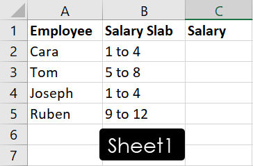
• In Sheet1 , I got employee names, salary slabs, and salary columns. I must import the salaries of the employees from a database of salary slabs and actual salaries in Sheet2 .

• In cell C2 , I’m entering the following formula that uses INDEX and MATCH to pull the correct data from Sheet2 to Sheet1 :

• Now, I can drag the fill handle down column C to populate salaries for other employees.

When using the formula in your own dataset, modify it as outlined below:

• Sheet2! : Change it to the exact worksheet name in your workbook.
• $A$2:$A$4 : Modify the cell range according to the dataset that needs indexing.
• B2 : It’s the reference data by matching which Excel will pull data from the indexed dataset.
• $B$2:$B$4 : This is the look-up value or array. Modify it according to your own dataset.

Pull Data From a Different Workbook

When you’re pulling data from a different workbook than the one you’re working on, you just need to include its name in the same formula shown above. Now, there could be two situations. One, where you’ve opened the source workbook, and the other where you didn’t open the source workbook.

If the source workbook is also open, use this formula:

If the source Excel file isn’t open but it’s on the same computer, use the following formula instead:

The difference in the above two formulas is the mention of the complete location of the source workbook in the internal storage of the PC.

When creating the link between two workbooks for the first time, keep both of them open and use the first formula that doesn’t show the address of the source Excel workbook. Now, the next time, if you keep the source workbook closed, Excel will add the directory address to the formula if the workbook isn’t open.

Pull Data Using Fill Handle

Another easy way to pull data without any formula in Excel is by using the fill handle. Suppose, you need to often copy a dataset from one worksheet to the other.

Here’s how you can do it in a few clicks without remembering any worksheet or workbook referencing convention in Excel:

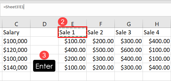
• Double-click the destination cell and enter an equal sign ( = ).
• Now, go to the source worksheet or workbook and highlight the starting cell of the table or dataset.
• Hit Enter .
• Excel will take you to the destination worksheet and pull the selected cell data from the source.

• Now, use the fill handle vertically to populate the data from the source worksheet or workbook.

• Then, drag the fill handle horizontally to get the rest of the dataset or table.

• You might see some cells containing the number 0 . This represents the blank cells in the source worksheet or workbook.
• Use the fill handle again to adjust the cell ranges horizontally and vertically to erase zeroes.

Alternatively, use the above Excel VBA code to get rid of zeroes.

Here’s how you can quickly use the above code:

• Right-click on the worksheet name.
• Click View Code on the context menu.

• Copy and paste the above VBA script inside the blank module.
• Click the Save button.

• Now, press Alt + F8 to bring up the Macro dialog box and run the RemoveZeros macro.

Pull Data Using Named Range

Named range in Excel allows you to define a name for a table or dataset within a workbook. Now, you can refer to the name instead of the cell range to pull data from a different worksheet or workbook. Find below the steps to creating and linking a named range to import data to a worksheet:

• Highlight the dataset in the source worksheet or workbook.
• Click the Formulas tab on the Excel ribbon menu .
• Inside the Defined Names commands block, click Define Name .
• In the New Name dialog box, enter a name you can remember for the highlighted dataset into the Name field.
• Click OK to complete the process.
• Now, go to the destination cell in a worksheet and enter the above formula.

• Press Enter or Ctrl + Shift + Enter to pull data from another sheet in Excel.

Copy Data From Another Sheet

The easiest way to pull data from another worksheet or workbook is the copy-paste method. However, this method might not be convenient when you need to pull a large dataset. Not to mention, manual copying and pasting comes with the risk of human error.

Find below two ways to automate the copy-paste process in Excel to pull data from a source worksheet:

Copy Data Between Worksheets Using VBA

• Press Alt + F11 to call the Excel VBA Editor interface.
• Click the Insert menu and choose Module .
• Into the new module, copy and paste this VBA script :
• Click the Save button and close the VBA Editor.

• Now, bring up the Macro dialog box by pressing Alt + F8 keys.
• Select the PullDataFromSheet4ToSheet3 macro and hit the Run button.

Excel will copy the source data into the destination worksheet instantly. Find below how to customize the VBA macro to make it work for your worksheet:

• Sheet4 : It’s the source of data so modify the sheet name.
• Sheet3 : It’s the destination where Excel will pull data from the source.
• A1:H5 : This is the cell range of the source data that Excel will copy. Change it to include more or less data according to your source worksheet.
• A1 : It’s the first cell in the destination worksheet from which Excel will start pasting the copied data. You can modify it if you want to.

Copy Data Between Sheets Using Office Scripts

Suppose you want to automate the pull data process from one worksheet to another on Excel online app. Since VBA won’t work there, you can use Office Scripts. Find below the steps you should try:

• Go to the destination worksheet and click Automate on the Excel ribbon .
• Click New Script inside the Scripting Tools commands block.
• The Code Editor panel will appear on the right side of Excel.
• There, copy and paste the above Office Scripts code.
• Click the Save script button to save the code.
• Now, hit the Run button to pull data from another worksheet in Excel automatically.

Here’s how you can personalize the above Office Scripts code.

• Change all the occurrences of Sheet3 with the actual worksheet name of the source data.
• Similarly, modify all the occurrences of Sheet4 according to the destination worksheet name.
• Replace "E1" in the code element sheet4.getRange("E1") with a cell address from which you want to start pasting the source data.
• Replace the cell range "E1:H5" in the code element selectedSheet.getRange("E1:H5") with the actual source data range, like "A1:F100" , "B2:E10" , etc.

Office Scripts is only available on Microsoft 365 subscription Business Standard or better. Also, you need an internet connection if you want to use Office Scripots in Excel for Microsoft 365 desktop app. If you see the Automate tab on Excel, you can use Office Scripts.

Pull Data From Another Sheet Using Power Query

Power Query is another cool database querying tool of Excel that lets you import data from different worksheets of the same workbook or from a different workbook.

When pulling data from Excel files using Power Query , you can make the process more efficient by using named ranges. Refer to the named range creation process explained above to give a name to the source dataset or table.

Once you’ve got the Defined Name you need, follow these steps:

• Go to the destination worksheet and click the Data tab.
• Hit the Get Data button and choose From Excel Workbook .

• Navigate to the source workbook and select it in the Import Data dialog box.
• Click Import to load the content of the workbook in the Navigator dialog box.

• Select the named range from the left-side panel.
• Now, click the drop-down arrow of the Load button and choose Load To .

• Select Existing worksheet on the Import Data dialog box and click OK .

Excel will instantly import the selected named range as a table with active filters. Select all the column headers and press Ctrl + Shift + L to deactivate filters.

Conclusions

So, now you know all the cool and intuitive methods to pull data from another sheet in Excel. You can also apply these steps to import data from a worksheet in a different workbook on your computer.

If you’re just starting your Excel journey, you can use the sheet and cell referencing method or the fill handle method. These are suitable for small datasets.

If you’re an expert-level Excel user and don’t mind writing a few lines of codes, use the Excel VBA and Office Scripts-based methods. These allow you to automate the whole process.

Finally, if you need to transform the source data into an organized structure before importing into the active worksheet, use the Power Query-based method. It comes with a visual interface so you can perform complex data management activities without writing codes.

About the Author

Subscribe for awesome Microsoft Excel videos 😃

John MacDougall

I’m John , and my goal is to help you Excel!

You’ll find a ton of awesome tips , tricks , tutorials , and templates here to help you save time and effort in your work.

• Pivot Table Tips and Tricks You Need to Know
• Everything You Need to Know About Excel Tables
• The Complete Guide to Power Query
• Introduction To Power Query M Code
• The Complete List of Keyboard Shortcuts in Microsoft Excel
• The Complete List of VBA Keyboard Shortcuts in Microsoft Excel

Related Posts

What is an Absolute Reference in Excel?

May 10, 2024

Wondering what is an absolute reference in Excel? Read this essential Excel...

What Does $ Mean in Excel?

May 9, 2024

What does $ mean in Excel? Read on to learn everything you need to know about...

7 Way to Unprotect a Sheet in Microsoft Excel

May 8, 2024

Want to learn how to unprotect Excel sheets? Read this Microsoft Excel...

In the early example you did not explain why there was a ,0 at the end of the formula. It appeared without explanation. =INDEX(Sheet2!$A$2:$A$4,MATCH(B2,Sheet2!$B$2:$B$4,0))

This is an option for the MATCH function that tells it to find an exact match.

Submit a Comment Cancel reply

Your email address will not be published. Required fields are marked *

Save my name, email, and website in this browser for the next time I comment.

Submit Comment

This site uses Akismet to reduce spam. Learn how your comment data is processed .

Get the Latest Microsoft Excel Tips

Follow us to stay up to date with the latest in Microsoft Excel!

How-To Geek

How to link or embed an excel worksheet in a word document.

Sometimes, you want to include the data on an Excel spreadsheet in your Microsoft Word document.

Quick Links

What's the difference between linking and embedding, how to link or embed an excel worksheet in microsoft word.

Sometimes, you want to include the data on an Excel spreadsheet in your Microsoft Word document. There are a couple of ways to do this, depending on whether or not you want to maintain a connection with the source Excel sheet. Let's take a look.

You actually have three options for including a spreadsheet in a Word document. The first is by simply copying that data from the spreadsheet, and then pasting it into the target document. For the most part, this only works with really simple data because that data just becomes a basic table or set of columns in Word (depending on the paste option you choose).

While that can be useful sometimes, your other two options---linking and embedding---are much more powerful, and are what we're going to show you how to do in this article. Both are pretty similar, in that you end up inserting an actual Excel spreadsheet in your target document. It will look like an Excel sheet, and you can use Excel's tools to manipulate it. The difference comes in how these two options treat their connection to that original Excel spreadsheet:

• If you link an Excel worksheet in a document, the target document and the original Excel sheet maintain a connection. If you update the Excel file, those updates get automatically reflected in the target document.
• If you embed an Excel worksheet in a document, that connection is broken. Updating the original Excel sheet does not automatically update the data in the target document.

There are advantages to both methods, of course. One advantage of linking a document (other than maintaining the connection) is that it keeps your Word document's file size down, because the data is mostly still stored in the Excel sheet and only displayed in Word. One disadvantage is that the original spreadsheet file needs to stay in the same location. If it doesn't, you'll have to link it again. And since it relies on the link to the original spreadsheet, it's not so useful if you need to distribute the document to people who don't have access to that location.

Embedding a document, on the other hand, increases the size of your Word document, because all that Excel data is actually embedded into the Word file. There are some distinct advantages to embedding, though. For example, if you're distributing that document to people who might not have access to the original Excel sheet, or if the document needs to show that Excel sheet at a specific point in time (rather than getting updated), embedding (and breaking the connection to the original sheet) makes more sense.

So, with all that in mind, let's take a look at how to link and embed an Excel Sheet in Microsoft Word.

Linking or embedding an Excel worksheet into a Word is actually pretty straightforward, and the process for doing either is almost identical. Start by opening both the Excel worksheet and the Word document you want to edit at the same time.

In Excel, select the cells you want to link or embed. If you would like to link or embed the entire worksheet, click on the box at the juncture of the rows and columns in the top left-hand corner to select the whole sheet.

Copy those cells by pressing CTRL+C in Windows or Command+C in macOS. You can also right-click any selected cell, and then choose the "Copy" option on the context menu.

Now, switch to your Word document and click to place the insertion point where you would like the linked or embedded material to go. On Home tab of the Ribbon, click the down arrow beneath the "Paste" button, and then choose the "Paste Special" command from the dropdown menu.

This opens the Paste Special window. And it's here where you'll find the only functional different in the processes of linking or embedding a file.

If you want to embed your spreadsheet, choose the "Paste" option over on the left. If you want to link your spreadsheet, choose the "Paste Link" option instead. Seriously, that's it. This process is otherwise identical.

Whichever option you choose, you'll next select the "Microsoft Excel Worksheet Object" in the box to the right, and then click the "OK" button.

And you'll see your Excel sheet (or the cells you selected) in your Word document.

If you linked the Excel data, you can't edit it directly in Word, but you can double-click anywhere on it to open the original spreadsheet file. And any updates you make to that original spreadsheet are then reflected in your Word document.

If you embedded the Excel data, you can edit it directly in Word. Double-click anywhere in the spreadsheet and you'll stay in the same Word window, but the Word Ribbon gets replaced by the Excel Ribbon and you can access all the Excel functionality. It's kind of cool.

And when you want to stop editing the spreadsheet and go back to your Word controls, just click anywhere outside the spreadsheet.

Note: If you working on a Word document and want to include a spreadsheet that you haven't created yet, you can. You can actually insert an Excel Spreadsheet right from the Table dropdown menu on the Ribbon.

Related: How To Use Excel-Style Spreadsheets in Microsoft Word

See links between worksheets

Important:  This feature isn’t available in Office on a Windows RT PC. Inquire is only available in the Office Professional Plus and Microsoft 365 Apps for enterprise editions.  Want to see what version of Office you're using?

A great way to check for links between worksheets is by using the Worksheet Relationship command in Excel. If Microsoft Office Professional Plus 2013 is installed on your computer, you can use this command, found on the Inquire tab, to quickly build a diagram that shows how worksheets are linked to each other. If you don't see the Inquire tab in the Excel ribbon, see Turn on the Spreadsheet Inquire add-in .

Open the file that you want to analyze for worksheet links.

On the Inquire tab, click Worksheet Relationship .

The Worksheet Relationship Diagram appears, showing links between the worksheets in the workbook.

Need more help?

Want more options.

Explore subscription benefits, browse training courses, learn how to secure your device, and more.

Microsoft 365 subscription benefits

Microsoft 365 training

Microsoft security

Accessibility center

Communities help you ask and answer questions, give feedback, and hear from experts with rich knowledge.

Ask the Microsoft Community

Microsoft Tech Community

Windows Insiders

Microsoft 365 Insiders

Was this information helpful?

Thank you for your feedback.

How to Hyperlink to Cell in Same Sheet in Excel (5 Methods)

We’re going to show you 5 methods in Excel to create a hyperlink to a cell in the same sheet. To demonstrate our methods, we’ve taken a dataset with 2 columns: “Products”, and “Unit Sold”.

How to Hyperlink to Cell in Same Sheet in Excel: 5 Ways

1. using insert link in excel to hyperlink to cell in same sheet.

We’re going to use the “ Insert Link ” feature in Excel to Hyperlink to cell in the same Sheet .

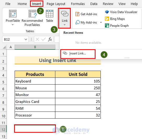
• Firstly, select cell B12 .
• Secondly, from the Insert tab >>> Link >>> select Insert Link…

Then, the “ Insert Hyperlink ” dialog box will appear.

• Thirdly, select “ Place in This Document ”.
• Select ‘ insert link’ from “ Or select a place in this document: ”
• Type “ Mouse ” in “ Text to display: ”
• Type B6 in “ Type the cell reference: ”.
• Finally, press OK .

We’ll see the text “ Mouse ” in cell B12 with link formatting .

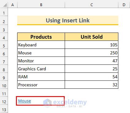
We can click on it, and it will select cell B6 . Thus, we’ve created an Excel Hyperlink in the same Sheet .

Read More: How to Add Hyperlink to Another Sheet in Excel

2. Hyperlink to Cell in Same Sheet by Implementing HYPERLINK Function

In this section, we’ll use the HYPERLINK function in Excel to create a Hyperlink to a cell in the same Sheet .

• Firstly, type the following formula in cell B12 .

The HYPERLINK function returns a clickable value. Here, we’ll get the link to cell C5 . Moreover, we’ve put a hash (“ # ”) to indicate within this Sheet . Then, we’ll display the second part in cell B12 which is “ Keyboard Sold ”.

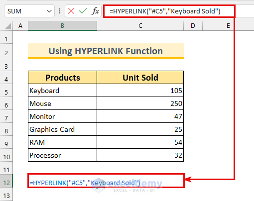
• Secondly, press ENTER .

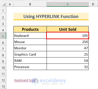
After that, we’ll see the text “ Keyboard Sold ” appear in cell B12 .

Again, we can click on this to go to cell C5 . Therefore, we’ve shown you yet another method of linking to a cell in the same Sheet .

Read More: How to Hyperlink Multiple Cells in Excel

3. Using Combined Functions to Create Dynamic Hyperlink to Cell in Same Sheet

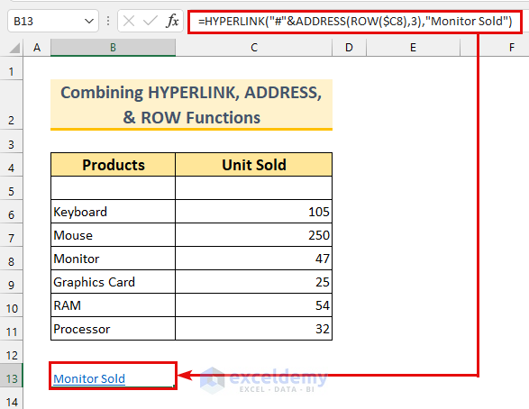
For the third method, we’ll use the ADDRESS , ROW , and HYPERLINK functions to create a dynamic link to a cell in the same Sheet . This means, that if we delete or insert rows or columns in the dataset, our formula will not break. Moreover, notice there is a blank row in our dataset.

• Firstly, type the following formula in cell B13 .

Formula Breakdown

• Output: {“$C$8”}.
• The ROW function returns the row number of a cell . Cell C8 will return 8 . Moreover, the ADDRESS function returns the location of a cell reference . Here, we’re denoting the C column by giving the value 3 in the formula. Thus we’ve got the output.
• Output: “Monitor Sold” .
• The HYPERLINK function returns a clickable value. Here, we’ll get the link to cell C8 . Moreover, we’ve put a hash (“ # ”) to indicate within this Sheet . Then, we’ll display the second part in cell B13 which is “ Monitor Sold ”.

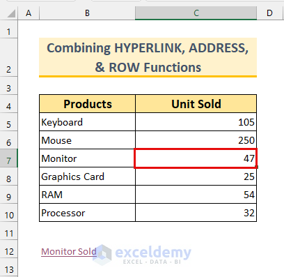
Then, we’ll see the output as described in the formula breakdown part.

We can click on that value to go to cell C8 . However, notice there is an empty row , we can delete blank rows to verify our dynamic formula still works.

• Finally, remove Row 5 .

If we click on the text “ Monitor Sold ”, we will select cell C7 now. Therefore, our formula works flawlessly.

Read More: How to Create Dynamic Hyperlink in Excel

4. Hyperlink to First Matched Cell in Same Sheet in Excel

In this section, we’ll use the CELL , INDEX , and MATCH functions to create a Hyperlink to the first matched values in the same Sheet .

• Output: 2 .
• The MATCH function is used to find the position of a value. Here, we’re looking for the value “ Mouse ” in the cell range B5:B10 . Moreover, we’ve put the 0 for exact matching.
• Output: “Mouse” .
• The INDEX function returns a value from a range. Here, we’re getting the value from the second row from the cell range B5:B10 which is cell B6 .
• Output: “$B$6” .
• The CELL function returns information about a cell . Here, we’ve set out info_type as “address” . This will return the first occurrence of the text “ Mouse ” in our range which is cell B6 .
• The HYPERLINK function returns a clickable value. Here, we’ll get the link to cell B6 . Moreover, we’ve put a hash (“ # ”) to indicate within this Sheet . Then, we’ll display the second part in cell B12 which is “ Mouse ”.

If we click on the text “ Mouse ”, we will select cell B6 . Thus, we’ve shown you yet another formula to Hyperlink to a cell in the same Sheet .

5. Creating Hyperlink to Cell in Same Sheet from a Value

For the last method, we’re going to create Hyperlinks to cells in the same Sheet from values by using the HYPERLINK and VLOOKUP functions. Moreover, we’ve adjusted our dataset a bit for this.

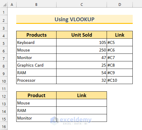
• Firstly, type the following formula in cell C13 .
• Output: “#C6” .
• Firstly, we’re looking for the value in cell B13 which is “ Mouse ”.
• Secondly, we’re setting our range in B5:D10 .
• Thirdly, we’ll extract the value from column 3 which is the “ Link ” column .
• Finally, we’re putting 0 to find an exact match .
• Output: “Mouse Sold” .
• The HYPERLINK function returns a clickable value. Here, we’ll get the link to cell C6 . Moreover, there is a hash (“ # ”) to indicate within this Sheet . Then, we’ll display the second part in cell B13 joined by the text “ Sold ” which is “ Mouse Sold ”.

• Finally, use the Fill Handle to AutoFill the formula .

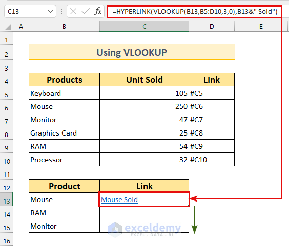
We can click on any of the Hyperlinks to go to their respective “ Unit Sold ” values in the dataset. In conclusion, we’ve achieved our goal of creating a Hyperlink to a cell in the same Sheet .

Read More: Excel Hyperlink to Cell in Another Sheet with VLOOKUP

Practice Section

We’ve provided practice datasets for each method in the Excel file.

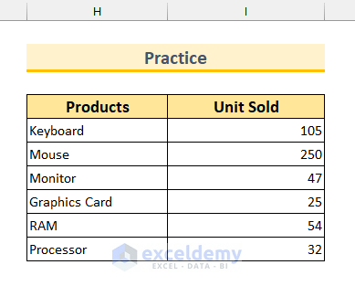
Download Practice Workbook

We’ve shown you 5 methods of Excel Hyperlink to cell in the same Sheet. If you face any difficulties in understanding any of the methods, feel free to comment below. Thanks for reading, keep excelling!

Related Articles

• How to Combine Text and Hyperlink in Excel Cell
• Excel Hyperlink to Another Sheet Based on Cell Value
• How to Create a Drop Down List Hyperlink to Another Sheet in Excel
• How to Edit Hyperlink in Excel
• How to Copy Hyperlink in Excel
• How to Convert Text to Hyperlink in Excel
• How to Create Button to Link to Another Sheet in Excel

<< Go Back To Create Hyperlink in Excel | Hyperlink in Excel  | Linking in Excel  |  Learn Excel

What is ExcelDemy?

Tags: Create Hyperlink in Excel

Rafiul Haq worked as an Excel and VBA Content Developer in Exceldemy for over two years and published almost 200 articles for the website. He is passionate about exploring new aspects of Excel and VBA. He received his Bachelor of Science in Mechanical and Production Engineering (MPE) from the Islamic University of Technology. Rafiul furthered his education by obtaining an MBA in Finance from the Institute of Business Administration (IBA) at the University of Dhaka. Apart from creating... Read Full Bio

Leave a reply Cancel reply

ExcelDemy is a place where you can learn Excel, and get solutions to your Excel & Excel VBA-related problems, Data Analysis with Excel, etc. We provide tips, how to guide, provide online training, and also provide Excel solutions to your business problems.

Contact  |  Privacy Policy  |  TOS

• User Reviews
• List of Services
• Service Pricing

• Create Basic Excel Pivot Tables
• Excel Formulas and Functions
• Excel Charts and SmartArt Graphics
• Advanced Excel Training
• Data Analysis Excel for Beginners

Advanced Excel Exercises with Solutions PDF

• Apple Watch
• Accessories
• Digital Magazine – Subscribe
• Digital Magazine – Info
• Smart Answers
• Let Loose iPad event
• New iPad Pro
• New iPad Air
• Best Mac antivirus
• Best Mac VPN

When you purchase through links in our articles, we may earn a small commission. This doesn't affect our editorial independence .

How to recover unsaved Excel files on Mac in 4 ways

You’ve spent hours working on an Excel workbook on a MacBook, but now it’s gone. Or, when you exit an Excel file, you unintentionally select “Don’t Save”. Is this to say that your entire effort has been in vain? This article systematically explains how to recover lost Excel files on a Mac . With our 4 methods, you can recover unsaved Excel files quickly.

After selecting the “Don’t Save” option or shutting down the MacBook without saving files, the Excel file vanishes on the Mac. Then, you should apply data recovery as quickly as possible; there is still a good chance you can recover your lost Excel document.

Method 1. Recover unsaved Excel files on a Mac with software

The most convenient method is to use professional Mac recovery software to restore the unsaved Excel files. EaseUS Data Recovery Wizard for Mac can help you find unsaved Excel files and deleted documents with a single click.

It can restore an Excel document saved on a Mac and works well with other Microsoft files, including Word, Excel, PowerPoint, and more. Users without experience can recover lost files on Mac with EaseUS data recovery software. Even if the Mac’s Excel files are permanently deleted, it can restore them.

Step 1. Select the disk

Launch EaseUS Data Recovery Wizard for Mac, hover your mouse over the device where you lost an unsaved file, and then select “Search for lost files”.

Step 2. Choose unsaved Excel files

After the scan, click “Type” and expand “Unsaved Documents”. Click on the file type you lost without saving, such as “Excel”.

Step 3. Preview and recover unsaved Excel files

Double-click to preview your unsaved file, select the appropriate version, and click “Recover” to save it to a different secure location on your Mac.

Method 2. Try the finder’s search feature on Mac

Finder on Mac features a built-in search capability that allows you to find files in any folder on your Mac. It is helpful when you want to retrieve vanishing desktop files or show hidden files on a Mac .

Step 1. Open the Finder and click the Search icon in the upper right corner.

Step 2. Enter the name of the file. The finder will begin searching automatically.

Step 3. If you do not know the name of the missing Excel file, you can instruct Finder to display all Excel files stored on your Mac by typing “.xls” or “.”xlsx” and picking the Microsoft Excel Workbook under Kinds.

Method 3. Recover unsaved Excel files from the Mac’s temporary folder

If you’ve been working with Microsoft, you may be familiar with temporary files on Mac. Similar to Word documents, Excel files generate temporary folders. As a result, you can retrieve the unsaved Excel files from these folders. Check out the following steps:

Step 1. Launch Terminal from the “Applications > Utilities” folder on your Mac.

Step 2. Type the command open $TMPDIR and press “Enter” to find the temporary folder.

Step 3. Select the unsaved Excel temporary files you want to recover. They are often shown as files with “.tmp” extensions. Right-click and open them with Excel on your Mac to see if you can read the files.

Method 4. Recover unsaved Excel files from AutoSave on Mac

In addition to rescuing unsaved Excel files from temporary files, Microsoft has launched the AutoRecover feature, which automatically saves copies and easily recovers files in Office for Mac .

Excel would allow you to recover the automatically saved copy of your worksheet following a closing. If Excel does not display the last opened file, check the AutoRecover folder manually:

Step 1. Launch Finder on your Mac Step 2. Type /Users/username/Library/Containers/com.microsoft.Excel/Data/Library/Preferences/AutoRecovery in the search box, and click “Go” to access the Excel AutoRecovery folder.

Step 3. You can then manually move the unsaved Excel file to a secure location on your Mac. When the AutoRecover function is activated, you can recover an unsaved Excel file on a Mac after a crash or unintentional closing by simply relaunching Excel and selecting the file from the list of recoverable documents.

Recover Unsaved Excel Files on Mac FAQs

Here are 3 questions users also want to learn about recovering unsaved Excel files from Mac:

How can I recover lost Excel on a Mac without Autorecovery?

If you have not enabled the AutoSave option on Mac, you can find the lost Excel’s previous version in the Time Machine backup:

Step 1. Click the Time Machine icon and enter it.

Step 2. Open the folder where the Excel document should be stored

Step 3. Return to a day, week, or month to see if your file remains.

Step 4. Select the appropriate backup version and search for the missing file.

How do I recover deleted Excel files on Mac?

Advanced data recovery software or iCloud backups can recover a deleted Excel spreadsheet from your Mac.

Here are the steps for using data recovery software:

Step 1. Run EaseUS Data Recovery Wizard for Mac and select where the destroyed Excel workbook was saved.

Step 2. Click “Search for Lost Files” to see all deleted files in the selected location.

Step 3. Select the deleted Excel spreadsheet and click “Recover” to retrieve it.

How can I return to a previous version of an Excel file on a Mac?

To revert an Excel file to its prior version, follow the instructions below:

Step 1.   Open “Excel” on your Mac.

Step 2. Select “File > Revert To”.

Step 3. Choose “Last Opened”, “Last Saved”, or “Previous Save” to revert an Excel to its prior version on Mac.

Losing a crucial unsaved Excel file can be sad, but it may not be permanent. In this post, we’ve covered four methods for recovering lost or unsaved Excel files, including showing them in Finder, trying data recovery software, recovering from temporary folders, and restoring from the AutoSave feature. 

At least one will likely come in handy. Follow the step-by-step instructions to select the best approach for Mac unsaved Excel recovery and restore your valuable workbooks. If you’ve deleted Excel files, restore them from the Trash or backup on Mac.