water pollution project observation

MAX-PLANCK-INSTITUT FÜR WISSENSCHAFTSGESCHICHTE Max Planck Institute for the History of Science

River sentinel/mollusc Corbicula fluminae (photo J.-C. Massabuau LEESA).

Observing and Making the Effects of Pollution Explicit

• The History of Scientific Observation
• Christelle Gramaglia

Unless exceptional events cause effects directly visible to the naked eye, air, and water pollution remain mostly imperceptible. The frequent absence of external signs when pollutants are present, and their ability to blend with other bodies, generate phenomena which are hardly discernible for who doesn’t possess the adequate equipment. Ozone in air and metallic pollution in water, for instance, cannot be noticed immediately. Furthermore, the physical and chemical properties of those contaminants contribute to produce specific moving geographies that escape our ordinary detection devices.

Until the end of the 1980s, the observation and monitoring of pollution rested on conventional chemistry methods that permitted to identify and assess concentrations of contaminants in the atmosphere, water, or sediments. If such analyses give indications on the presence or absence of one particular pollutant, they do not tell us its impact on living entities and natural environments, nor the effects of the accumulation of low doses, or the compound effects of several pollutants.

As a young and controversial discipline, ecotoxicology developed new observation instruments that allow to diagnose precisely the corruption of the quality of water or the degradation of specific environments. The observation techniques set up by ecotoxicology researchers rely on the sensitive and adaptative abilities of some living entities identified as "sentinel organisms" (providing bioindicators and biomarkers). In 1926, pioneer scientists started drawing up the map of atmospheric pollution by investigating lichen populations. At the end of the 1960s, the USA launched a sea water surveillance program by enrolling mussels in research protocols (Mussel Watch Program). If the presence and distribution of species provide important indications, the study of the biological responses those species produce in reaction to environmental perturbation supply information that are even more precise. Physiological, biochemical, and genetic tests are performed on "sentinel organisms" to reveal and make explicit the presence and impact of pollutants.

The living entities used by ecotoxicologists are not mere instruments or guinea pigs. They are rather partners that lend their sensitive qualities to the researchers. They are not interchangeable either. Each contaminated site and each type of pollutant require specific mediations, involving different experiments and "sentinel organisms." The information collected from several tests allows ecotoxicologists to develop observation devices that are so sharp that they can monitor the variations of toxicity in time and space.

This research project aimed at examining three main questions while studying the history of ecotoxicology and scientific controversies that have marked its evolution, and performed ethnographic fieldwork in two laboratories, in France and Germany.

• What was the evolution of observation methods and problems posed by the enrolment of living entities in research protocols? How doed the extension of laboratories, from the setting of observation devices to their use in situ, and the extension of the instruments to "sentinel organisms," contribute to the transformation of scientific practices? What are the constraints? How to account for the participation of those living entities as research auxiliaries?
• What were the steps permitting one to materialize and provide evidence of insidious pollution through the use of "sentinel organisms." Ecotoxicologists construct reduced models in their laboratory to target their experiments before testing them in the field. What are the differences between controlled observations made indoor and observations made in natural environments? How can they be scientifically related? What visualization methods are used? Has the status of evidential documents changed along the history of the discipline? What sort of evidence do they provide, and which type of rhetoric is then needed to transport them?
• What were the epistemological and political consequences of the emergence of new experimental devices marked by features that are mostly local and subject to great variations? It seems that each environment, each contaminated site, each type of pollutant, requires adapted testing protocols. At the same time, each pollution phenomenon contributes to produce its own propagation space. Then, ecotoxicological experiments reinforce the attachments between scientists, specific places, some pollutants and species. What are the obstacles to the standardization and implementation on a large scale of those new observation and monitoring instruments? How do local claims actually transform into general? What are the consequences for our conception of objectivity and politics?

Publication

Gramaglia, C. 2005. "River Sentinels: Finding a Mouth for the Lot River." In B. Latour & P. Weibel (eds), Making Things Public. Atmospheres of Democracy. Cambridge: ZKM & MIT Press.

• Chemical & Physical Sciences
• Earth & Environmental Sciences
• Life Sciences
• Medicine & Health
• Observation & Experiment

• Reference Manager
• Simple TEXT file

People also looked at

Original research article, analysis of water pollution using different physicochemical parameters: a study of yamuna river.

• 1 Department of Electronics and Communication Engineering, Faculty of Engineering and Technology, SRM Institute of Science and Technology, Delhi- NCR Campus, Ghaziabad, India
• 2 Department of Computer Science and Engineering, Gandhi Institute of Engineering and Technology University, Gunupur, India
• 3 School of Computer Engineering, Kalinga Institute of Industrial Technology Deemed to Be University, Bhubaneswar, India
• 4 Department of Civil, Environmental and Natural Resources Engineering, Lulea University of Technology, Lulea, Sweden
• 5 Department of Electronics and Communication Engineering, Krishna Institute of Engineering and Technology, Group of Institutions, Ghaziabad, India
• 6 Department of Computer Science, SRM Institute of Science and Technology, NCR Campus, Ghaziabad, India
• 7 Department of Applied Sciences and Humanities, Teerthankar Mahaveer University, Moradabad, India
• 8 Institute of Research and Development, Duy Tan University, Da Nang, Vietnam
• 9 Geotechnical Engineering and Artificial Intelligence Research Group (GEOAI), University of Transport Technology, Hanoi, Vietnam

The Yamuna river has become one of the most polluted rivers in India as well as in the world because of the high-density population growth and speedy industrialization. The Yamuna river is severely polluted and needs urgent revival. The Yamuna river in Dehradun is polluted due to exceptional tourist activity, poor sewage facilities, and insufficient wastewater management amenities. The measurement of the quality can be done by water quality assessment. In this study, the water quality index has been calculated for the Yamuna river at Dehradun using monthly measurements of 12 physicochemical parameters. Trend forecasting for river water pollution has been performed using different parameters for the years 2020–2024 at Dehradun. The study shows that the values of four parameters namely, Temperature, Total Coliform, TDS, and Hardness are increasing yearly, whereas the values of pH and DO are not rising heavily. The considered physicochemical parameters for the study are TDS, Chlorides, Alkalinity, DO, Temperature, COD, BOD, pH, Magnesium, Hardness, Total Coliform, and Calcium. As per the results and trend analysis, the value of total coliform, temperature, and hardness are rising year by year, which is a matter of concern. The values of the considered physicochemical parameters have been monitored using various monitoring stations installed by the Central Pollution Control Board (CPCB), India.

Introduction

Due to historical, geographical, religious, political, and sociocultural reasons, India has a unique place in the world Agarwal et al., 2016 . Pollution-causing activities have caused severe changes in aquatic environments over the last few decades. Serious questions have been raised in context to the safe use of river water for drinking and other purposes in recent times. Numerous contaminants are playing a major role in polluting the river water. It is one of the main concerns for most of the metropolitan cities of developing nations. Rivers play a vital role in shaping up the natural, cultural, and economic aspects of any country ( Rafiq, 2016 ). The Yamuna river is one such river. The Yamuna river provides sustenance to ecology and is therefore considered holy by the people of India. It derives from the glacier called Yamunotri in the Himalayan ranges. States through which the Yamuna river flows are the Uttarakhand, Himachal Pradesh, Uttar Pradesh, Haryana, and Delhi. The Yamuna river is also divided into several tributaries such as the Hindon, Tons, Giri, Rishiganga, Hanuman Ganga, Sasur Khaderi, Chambal, Betwa, Ken, Sindh, and Baghain as it is flowing through several cities. These cities are the Yamuna Nagar, Delhi, Faridabad, Mathura, Agra, Etawah, and Prayagraj. It is a tributary of the river Ganges in India. Two of them together have had substantial importance in shaping up the history and geography of our country. The river on which our research primarily focuses is the Yamuna river. It passes through several states such as Uttar Pradesh, Himachal Pradesh, Uttarakhand, Haryana, and Delhi. It has a length of approximately 1,380 km. More than 600 lakh people are dependent on their living and income on this river ( Census Reports of India 2001 , 1971–1991 ). Such is the greatness of this river. Our research is based on the Yamuna river in Dehradun in Uttarakhand.

The process, in which the people from rustic areas shift to the town areas in search of a brighter future, thus resulting in a drastic increment in the population of people living in cities, is called urbanization. As a result, the number of cities and towns increases exponentially. There is an atrocious amount of stress on the weakening natural resources. As it is, the natural resources are facing major deterioration issues considering the unthoughtful plundering by the people. In the last few decades, the rate of spread in various segments of the world has been unprecedented and unimaginable. The proportion of the rate of infrastructure expansion has not been able to match up to the pace of urbanization in most cities. The amplified requirement of water, deficiency of sewage facilities, and scarce wastewater treatment facilities rigorously affect the water resources, and change the environment and ecology. Agricultural lands, rural unpaved areas, and natural wetlands are converted into paved and impervious urban areas, during urbanization. Augmented impervious land surface in urbanized areas leads to severe and radical changes in the natural order of things ( Ahmad et al., 2017 ). There has been a drastic decline in the Yamuna river water quality since the last few years. The water is highly polluted, and it is a joint responsibility of the government and all the citizens to make sure that the Yamuna river is clean again. The primary step toward understanding and deliberating about the sorts of water pollution and developing effective reduction strategies is monitoring ( Marale, 2012 ). Physical, chemical, and biological compositions determine the quality of water ( Allee and Johnson, 1999 ). The substances such as heavy metals, pesticides, detergents, and petroleum form the chemical composition ( Tiwari et al., 2020 ). Turbidity, color, and temperature comprise the physical composition, whereas the biological arrangement includes pigments and planktons. Observation and analysis of these water quality parameters need sampling from extensively distributed locations, which is time consuming and requires a lot of field and lab efforts to come up with statistical results ( Wang et al., 2004 ; Icaga, 2007 ; Kazi et al., 2009 ; Amandeep, 2011 ; Duong, 2012 ; Singh et al., 2013 ; Nazeer and Nichol, 2015 ; Shi et al., 2018 ).

Conventionally, monitoring-based methods are used to find out the water quality parameters. They involve wide-ranging field sampling and expensive lab analysis, which is time inefficient and can only be accomplished for areas that are smaller ( Song et al., 2012 ). Hence, these restraints and drawbacks make the conventional methods challenging for continuous water quality prediction at spatial scales ( Panwar et al., 2015 ; Chabuk et al., 2017 ). For observing and analyzing water quality parameters, such as turbidity, chlorophyll, temperature, and suspended inorganic materials, techniques, such as optical remote sensing, are being used ( Pattiaratchi et al., 1994 ; Fraser, 1998 ; Kondratyev et al., 1998 ). To calculate the measure of solar irradiance at varied wavelength bands reflected by the surface water, remote sensing satellite sensors are used ( Zhang et al., 2003 ; Dwivedi and Pathak, 2007 ; Girgin et al., 2010 ; Ronghang et al., 2019 ). Amplified demand for water, poor sewage facility, and insufficient wastewater management amenities, relentlessly affect the resources of water resources. Models such as hydrological models have been used to evaluate the effect of numerous factors in rain-related procedures of the cosmopolitan areas ( Trombadore et al., 2020 ). Knowledge and information about interconnections between climate, population, and ecology are essential for understanding and promoting sustainable development ( Sharma et al., 2020 ). It also requires better knowledge of equipment and methodical planning. Proper management will reduce the degradation of rivers ( Shukla et al., 2018 ). In this study, we focus on trying to find out contaminants in the river, finding the water pollution index, and subsequently enforcing measures to curb water pollution.

Contribution of the Study:

1. In the present study, water samples were collected every year from the Yamuna river canal in Dehradun, Uttarakhand, India.

2. The samples have been analyzed for 12 different physicochemical attributes like ph, BOD, COD, Total Coliform, Temp, DO, Alkalinity, Chlorides, Calcium, Magnesium, and Hardness as Calcium Carbonate and TDS.

3. The measurement of the water quality index has been taken into consideration for the years 2017, 2018, and 2019.

4. Forecasting the pollution trend for the Yamuna river water from 2016 to 2024.

Materials and Methods

Mathematical model.

In this research paper, the water sample of the Yamuna river is considered for analysis. The 12 physicochemical parameters in the water are studied and analyzed. The water sample of the Holy River called the Yamuna river is considered for a certain period. The ratio of water components mainly Temperature, Total Coliform, TDS, and Hardness are varied irregularly at various locations of India. Due to the abrupt changes in the water component, the water quality is also changed. In this research paper, a sampling distribution-based analytical model called Equipoise Evaluator (EE) is proposed for the discrete parameter value of the water components. The EE model is suitable to analyze random discrete parameters. The EE model can be applied for any kind of sample analysis where the analysis is based on sample molecules. To analyze the discrete sample in the form of the symmetric normal distribution for a particular location, the EE model is applied. In this research paper, the water sample varies based on the molecules of e water components. This EE model is also applicable for the analysis of metallurgy to detect the impurity of the metal. In this research paper, the EE model is deployed for the water sample of the Yamuna river.

Sampling distribution is proposed to transform the variable at different levels.

As per the linear transformation

Now, by applying the Jacobian transformation on a non-singular matrix M,

From Equation (2), the relational equation for all connected differential elements is defined as Equation (3)

As M is considered as an orthogonal matrix, hence Z = MW, which transformed into a quadratic form of preserving from the standard value.

To determine the dissimilarity distance from a standard sample value, the partitioning matrix is deployed.

Assume that matrix M is partitioned into qth numbers, then M i M j ′ = 0    ∀ i ≠ j .

As per the partitioning matrix, all q sub-matrices are orthogonal to each other except orthogonal themselves. Now, Equation (1) is rewritten as

where, M 1 ,…., M q are an exclusive subset of the tested variables.

Applying transformation in Equation (7)

where, B i = ( M i M i ′ ) - 1     a n d   η i = M i μ

Equation (8) determines the transformation of each partition into quadratic form with exclusive subsets of tested parameters. In this analysis, M is considered as fully orthogonal, with each row orthogonal to every other row. The result of transforming all the variables to test bed data variables of D is then,

It is considered that the water molecules of the sample water have symmetric normally distributed for a particular location. The mean of the water molecules is z ¯ = 1 q ∑ i = 1 q w i .

As per orthogonal transformation

where u 1 = q z ̄ and σ = u 1 2 + u 2 2 + . . . . + u q 2 .

u 1 and σ are independently distributed. The sample mean and sample variance of the experimented sample water are independently distributed.

Water Quality Index and Trend Analysis

The primary focus of this study is to measure and analyze the drastic changes in the Yamuna river water quality at Dehradun, Uttarakhand. Standardized and the universally accepted water quality index (WQI) has been adopted to measure the variation in water quality of the Yamuna river at the prime location of the study—Dehradun over 3 years. The standard method has been used to examine and evaluate the water quality for 12 Physicochemical parameters (TDS, Chlorides, Alkalinity, DO, Temperature, COD, BOD, pH, Magnesium, Hardness, Total Coliform, and Calcium). In this study, the water quality index has been calculated using the different Physicochemical parameters documented and verified from the monitored locations. The water quality index (WQI) is stated by

where Ii signifies the ith water quality parameters, the weight associated and related to the parameters is denoted by Wi, and p notifies us about the number of water quality parameters. This WQI is based on the index introduced by the NSF (National Sanitation Foundation) ( Bhutiani et al., 2016 ). This index is established by the Central Pollution Control board with different advancements in terms of water quality criteria. The Water quality index is supported and developed by the National Sanitation Foundation (NSF) ( Brown et al., 1970 ). It is also known as NSF-WQI. This water quality index is denoted as

where P denotes the ith parameter measured values, quality rating is denoted by q i , and the relative weight of the ith parameters is denoted by w i .

The water quality index arithmetic index was presented ( Cude, 2001 ). It is a very popular and standard method used by many investors and researchers in their studies ( Ramakrishniah et al., 2009 ; Ahmad et al., 2012 ).

In this study, the quality rating can be calculated using the following equation:

where q i signifies the ith parameter quality rating for n water quality parameters, water.

The quality parameters' actual and definite value is denoted by V actual , the parameters ideal value is symbolized by V ideal , and the standard value of the parameters, which is suggested by the WHO, is denoted by V standard . The ideal values for DO and pH are 14.6 and 7 mg/L, whereas for the other parameters, it is equal to zero. After the calculation of quality rating, (relative weight), Wi has to be calculated by inversing the standard value of the parameter. Finally, the following equation was used to calculate the overall water quality index (WQI):

Here, signifying the relative weight and quality rating is symbolized by Wi and qi .

Trend Analysis

In this study, to forecast the pollution trend analysis, the linear regression model has been used. According to the linear regression model, the relationship between the two variables a and b can be expressed as:

Where x and y are the model parameters, which are known as regression coefficients, and B is the dependent variable. A is known as an independent variable, and € is the error variable. For making a prediction using a linear regression model is

The parameters x and y are calculated using the following equations:

Methodology

The flow chart for the methodology used is shown in Figure 1 . The water quality index is calculated using the weight arithmetic water quality index method, which has been discussed in the Water Quality Index and Trend Analysis section.

Figure 1 . Flow chart for the methodology used.

The value of the water quality index has been compared with the standard values of WQI, which is shown in Table 1 . The water quality rating is divided into five categories. The range from 0 to 25 is coming under (A) grading with excellent water quality, the range from 26 to 50 is for grading (B) with good water quality, and respectively, (C), (D), and (E) gradings are categorized for different WQI values ( Chauhan and Singh, 2010 ).

Table 1 . The standard values of water quality index (WQI) using weight arithmetic water quality index method.

Dataset Collection

The most populous city of Uttarakhand is Dehradun also spelled Dear Doon. It is the capital of Uttrakhand, which is one among the 28 states in India ( Figure 2 ). It is famous for its Doon Basmati Rice. Dehradun city has famous institutions like IMA (Indian Military Academy) regarded as one of the best officer training academies in India, Forest Research Institute, Indian Institute of Petroleum, and the famous ONGC training institute. This city is also famous among the tourists. It has many adventurous activities like rafting, bungee jumping, paragliding, etc. ( Rafiq, 2016 ). The city is located about 255 km from New Delhi and 168 km from Chandigarh. The climate condition of Dehradun is humid, subtropical, and a summer temperature can reach a maximum of 44°C. This city is also located very close to Nainital, which has the famous Jim Corbett National Park attracting many tourists ( Bhutiani et al., 2015 ).

Figure 2 . Map for considering location for Yamuna, Dehradun ( https://www.bcmtouring.com/forums/thread ).

The present study was undertaken for a period of 3 years from 2017 to 2019 to check the water quality analysis for the physicochemical attributes below. In the present study, water samples were collected on a yearly basis from the Yamuna river canal in Dehradun, Uttarakhand, India. The samples were analyzed for 12 different physicochemical attributes like ph, BOD, COD, Total Coliform, Temp, DO, Alkalinity, Chlorides, Calcium, Magnesium, and Hardness as Calcium Carbonate, and TDS ( Tyagi et al., 2020 ). The Yamuna river plays a very crucial role in Dehradun's geography. The Yamuna river is severely polluted and needs urgent revival. The river passes through Uttarakhand. Uttarakhand has always been a tourist spot and experiences heavy tourists perennially, and Dehradun, being the capital city, also bears the brunt. The Yamuna river in Dehradun is polluted due to the exceptional tourist activities. Dehradun is also famous for the Kumaoni Holi, Jhanda Fair, Tapkeshwar Mela, and Bissu Mela. A lot of waste materials are dumped into the Yamuna river, and they contaminate the river. Water might be untreated for long spans of time. Also, a lot of industries–primarily biotechnology and food processing, are set up in Dehradun; they also mindlessly dump their waste in the Yamuna river. Industrial waste is not fully responsible for the pollution, but some poor sewage systems and human activities are also responsible for it ( Bhutiani and Khanna, 2007 ).

Dehradun is a home to many agricultural and horticulture activities such as rice, litchi, and tea plantations. Agricultural waste also plays a major role in polluting the Yamuna river in Dehradun. The pollution is also increased by the excessive usage of insecticides and pesticides ( Tiwari et al., 2020 ). There are also people who wash their clothes, utensils, and defecate in or around the river, thus leading to pollution. The stretch of the Yamuna river in Dehradun thus has a lot of coliform bacteria. Government projects such as road construction might also be responsible for dumping waste, although rules have been drastically upgraded in the last two decades or so. Some cattle washing activities and religious activities also polluted the Yamuna river ( Bhutiani et al., 2018 ).

Results and Discussion

The study aims to examine the alteration in the quality of water of the Yamuna river at Dehradun in the year 2017. Water quality index (WQI) is going to be used in the study so that the changes and variations in the quality of water of the Yamuna river can be measured. The conventional method by which inspection can be done for the water quality has 12 physicochemical parameters (TDS, Chlorides, Alkalinity, DO, Temperature, COD, BOD, pH, Magnesium, Hardness, Total Coliform, and Calcium). These parameters will be measured carefully, and their respective value will be found. So, the standard value and observed value will be compared with each other, and the variation is going to be measured between them. By this variation, identification of the quality of water can be done.

Measurement of Physicochemical Parameters at Dehradun for 2017

Water samples have been taken at different months for the year 2017 ( Table 2 ). The mean and standard deviation for the measured values have been also calculated. The mean is the number found by summing every data point and dividing by the number of data points. It is also called average. The standard deviation is defined as the number that is going to tell about the measurements for a group that is spread out from the mean or expected value. A low standard deviation signifies that many numbers are very close to the mean ( Bisht et al., 2017 ). A high standard deviation signifies that the numbers are very much spread out. So, the accurate value for the quality of water can be found out easily using this.

Table 2 . Physicochemical parameters and water quality analysis at Dehradun for 2017.

The maximum value of pH is in the month of January when the water is a little more basic, and the minimum value is in July when it is less basic. The mean pH is 7.735, and the standard deviation is 0.086986589. The maximum value of the biochemical oxygen demand (BOD) is in January, which indicates more polluted water, and the minimum value is in the months of April, July, and October, which indicates less polluted water. The mean of BOD is 1.05, and the standard deviation is 0.1. The maximum value of COD is in January and October, which indicates a large quantity of oxidizable organic materials in the sample, and the minimum value is in April and July which indicates a lesser quantity of oxidizable organic materials in the sample. The mean COD is 5 and the standard deviation is 1.154700538.

The maximum value of Total Coliform is in July, which indicates that the water-borne illness is increased, and the minimum value is in October which indicates that the water-borne illness is decreased. The mean of Total Coliform is 65, and the standard deviation is 17.32050808. The maximum value of Temp is in July, which indicates increased chemical reactions generally, and the minimum value is in January, which indicates decreased chemical reactions. The mean of Temp is 17.75, and the standard deviation is 2.62995564. The maximum value of DO is in October, and the minimum value is in January, April, and July. The mean of DO is 8.7, and the standard deviation is 0.2. The maximum value of Alkalinity/visual titration CaCO 3 is in July, which indicates greater buffering capacity against pH changes, and the minimum value is in April, which indicates lesser buffering capacity against pH changes. The mean of Alkalinity/visual titration CaCO 3 is 64, and the standard deviation is 5.887840578. The maximum value of Chlorides is in July, which indicates body-related diseases, and the minimum value is in April and October. The mean of Chlorides is 5.75, and the standard deviation is 0.9574271078. The maximum value of Calcium as CaCO 3 is in July, which has a positive effect on the body, and the minimum value is in April, which has a lesser positive effect on the body. The mean of CaCO 3 is 41, and the standard deviation is 4.760952286. The maximum value of Magnesium as CaCO 3 is in July, which has a positive effect on the body, and the minimum value is in January, which has a lesser positive effect on the body. The mean of Magnesium as CaCO 3 is 32.5, and the standard deviation is 2.516611478. The maximum value of Hardness as CaCO 3 is in July, which has a good effect on the body, and the minimum value is in April. The mean of Hardness as CaCO 3 is 73.5, and the standard deviation is 6.191391874. The maximum value of TDS is in July, which specifies more toxic minerals, and the minimum value is in April, which specifies less toxic minerals. The mean of TDS is 83.75, and the standard deviation is 14.7507062. Water quality index (WQI) was used for the evaluation of the variation in the water quality of the Yamuna river at Dehradun over 3 years. The standard and prescribed methods have been used to analyze the water quality for 12 physicochemical parameters (TDS, Chlorides, Alkalinity, DO, Temperature, COD, BOD, pH, Magnesium, Hardness, Total Coliform, and Calcium). Calculations have been performed using the standardized formula and mathematical models. Detailed calculations and methodology have been used to find the water quality index as accurately as possible. The WQI of the Yamuna river in Dehradun for the year 2017 was 42.87 ( Table 2 ). According to WHO, the WQI should be below 60 for its quality to be at least fair. Here, it can be easily concluded that the Yamuna river is polluted, but it is still revivable. Developmental and maintaining efforts can be adopted to make the Yamuna river clean again and improve the WQI drastically.

Total coliform is positively correlated with CaCO 3 , chlorides, and hardness of CaCO 3 .Temp is positively correlated with the magnesium of CaCO 3 and TDS and negatively correlated with pH, BOD, and COD. DO is positively correlated with COD and negatively correlated with chlorides. Alkalinity is positively correlated with chlorides, TDS, hardness, and the magnesium of CaCO 3 and negatively correlated with pH. Chlorides are positively correlated with calcium and hardness of CaCO 3 and negatively correlated with pH and DO. Magnesium (CaCO 3 ) is positively correlated with hardness and TDS, and negative with pH, BOD, and COD. Hardness (CaCO 3 ) is positive for TDS, Chlorides, Magnesium, and negative for pH. TDS is negative for pH and positive for all. The dendrogram and graphical representation for physicochemical parameters at Dehradun for 2017 are plotted between the months (January, April, July, and October) and the parameters [TDS, Total Coliform (MPN/100 ml), Alkalinity/visual titration CaCO 3 , Hardness as CaCO 3 , Calcium as CaCO 3 , Magnesium as CaCO 3 , Temp, BOD, pH, DO, COD, and Chlorides] ( Figures 3 , 4 ).

Figure 3 . Dendrogram for physicochemical parameters at Dehradun for 2017.

Figure 4 . Graphical representation of physicochemical parameters at Dehradun for 2017.

Cluster 1 (blue) represents lightly polluted, and the parameters include TDS, Total Coliform (MPN/100 ml), Alkalinity/visual titration CaCO 3 , and Hardness as CaCO 3 . Cluster 2 (red) represents moderately polluted, and the parameters include Calcium as CaCO 3 , Magnesium as CaCO 3 , Temp, BOD, pH, DO, COD, and Chlorides. Cluster 3 (black) represents heavily polluted and the parameters include Total Coliform (MPN/100 ml), Alkalinity/visual titration CaCO 3 , Hardness as CaCO 3 , Calcium as CaCO 3 , Magnesium as CaCO 3 , and Temp.

Measurement of Physicochemical Parameters at Dehradun for 2018

Water samples have been taken in different months for the year 2018 ( Table 3 ). Mean and standard deviation for the measured values have been also calculated. The maximum value of pH is in October so the water is a little more basic, and the minimum value is in January, which means the water is less basic. The mean pH is 7.6325, and the standard deviation is 0.420585. The maximum value and minimum value of BOD are equal every month. The mean of BOD is 1, and the standard deviation is 0.

Table 3 . Physicochemical parameters and water quality analysis at Dehradun for 2018.

The maximum value of COD is in April indicating a large quantity of oxidizable organic material in the sample, and the minimum value is in January, July, and October indicating a lesser quantity of oxidizable organic materials in the sample. The mean of COD is 4.5, and the standard deviation is 1. The maximum value of Total Coliform is in July indicating the water-borne illness is increased, and the minimum value is in January, April, and October indicating the water-borne illness is decreased. The mean of Total Coliform is 50, and the standard deviation is 20. The maximum value of Temp is in July indicating increased chemical reactions generally, and the minimum value is in January indicating decreased chemical reactions. The mean of Temp is 18.25, and the standard deviation is 1.707825. The maximum value of DO is in April, and the minimum value is in January and July. The mean of DO is 8.85, and the standard deviation is 0.251661. The maximum value of Alkalinity/visual titration CaCO 3 is in July indicating higher buffering capacity against pH changes, and the minimum value is in April indicating lower buffering capacity against pH changes. The mean of Alkalinity/visual titration CaCO 3 is 64.5, and the standard deviation is 6.608076.

The maximum value of Chlorides is in January, July, and October indicating body-related diseases, and the minimum value is in April. The mean of Chlorides is 5.75, and the standard deviation is 0.5. The maximum value of Calcium as CaCO 3 is in July, which has a positive effect on the body, and the minimum value is in January, April, and October, which has a less positive effect on the body. The mean of CaCO 3 is 41.5, and the standard deviation is 3. The maximum value of Magnesium as CaCO 3 is in July, which has a positive effect on the body, and the minimum value is in April, which has a less positive effect on the body. The mean of Magnesium as CaCO 3 is 33, and the standard deviation is 2.581989. The maximum value of Hardness as CaCO 3 is in July, which has a good effect on the body, and the minimum value is in April. The mean of Hardness as CaCO 3 is 74.5, and the standard deviation is 5.259911. The maximum value of TDS is in July specifying the presence of toxic minerals, and the minimum value is in January specifying the presence of less toxic minerals. The mean of TDS is 87.5, and the standard deviation is 15.60983.

Water quality index (WQI) was used in the evaluation of the variation in water quality of the Yamuna river at Dehradun over 3 years. The standard and prescribed method has been used to analyze the water quality for the 12 physicochemical parameters (TDS, Chlorides, Alkalinity, DO, Temperature, COD, BOD, pH, Magnesium, Hardness, Total Coliform, and Calcium). Calculations have been performed using the standardized formula and mathematical models. Detailed calculations and methodology have been used to find the water quality index as accurately as possible. The WQI of the Yamuna river in Dehradun for the year 2018 was 40.47 ( Table 3 ). According to WHO, the WQI should be below 60 for its quality to be at least fair. Here, it can be easily concluded that the Yamuna river is polluted, but it is still revivable. Developmental and maintaining efforts can be adopted to make the Yamuna river clean again and improve the WQI severely. Moreover, it is a positive sign that the WQI of the Yamuna river has improved greatly for the year 2018 compared to the year 2017.

The dendrogram and graphical representation for the physicochemical parameters at Dehradun for 2018 are plotted between the months (January, April, July, and October) and also the parameters [TDS, Total Coliform (MPN/100 ml), Alkalinity/visual titration CaCO 3 , Hardness as CaCO 3 , Calcium as CaCO 3 , Magnesium as CaCO 3 , Temp, BOD, pH, DO, COD, and Chlorides] ( Figures 5 , 6 ). Cluster 1 (blue) represents lightly polluted and the parameters include Temp, BOD, pH, DO, COD, and Chlorides.

Figure 5 . Dendrogram for physicochemical parameters at Dehradun for 2018.

Figure 6 . Graphical representation of physicochemical parameters at Dehradun for 2018.

Cluster 2 (red) represents moderately polluted, and the parameters include Total Coliform (MPN/100 ml), Calcium as CaCO 3 , Magnesium as CaCO 3 , TDS, Alkalinity/visual titration CaCO 3 , Hardness as CaCO 3 . Cluster 3 (black) represents heavily polluted, and the parameters include BOD, pH, DO, COD, Chlorides, Total Coliform (MPN/100 ml), Alkalinity/visual titration CaCO 3 , Hardness as CaCO 3 , Calcium as CaCO 3 , and Magnesium as CaCO 3 .

Measurement of Physicochemical Parameters at Dehradun for 2019

Water samples have been taken in different months for the year 2019 ( Table 4 ). The mean and standard deviation for the measured values have been also calculated. The mean is the number found by summing every data point and dividing by the number of data points. Standard deviation is defined as the number that is going to tell about the measurements for a group that is spread out from the mean or expected value. Comparing the values of this year with those of the previous years leads to the outcomes being observed.

Table 4 . Physicochemical parameters and water quality analysis at Dehradun for 2019.

The maximum value of pH is in the month of January when the, water is a little more basic and the minimum value is in the month of October when the water is less basic. The mean pH is 7.6225, and the standard deviation is 0.411208. The maximum value of BOD is in July when there is a large quantity of polluted water, and the minimum value is in January, April, and October when there is less quantity of polluted water. The mean of BOD is 1.05, and the standard deviation is 0.1. The maximum value of COD is in July and October indicating a greater amount of oxidizable organic materials in the sample, and the minimum value is in January and April indicating a lesser amount of oxidizable organic materials in the sample. The mean of COD is 5, and the standard deviation is 1.154701. The maximum value of Total Coliform is in April indicating that water-borne illness is increased, and the minimum value is in January indicating that water-borne illness is decreased. The mean of Total Coliform is 182.5, and the standard deviation is 93.22911. The maximum value of Temp is in October indicating increased chemical reactions generally, and the minimum value is in January indicating decreased chemical reactions. The mean of Temp is 18.5, and the standard deviation is 1.290994. The maximum value of DO is in April, and the minimum value is in July. The mean of DO is 8.9, and the standard deviation is 0.258199. The maximum value of Alkalinity/visual titration CaCO 3 is in April indicating higher buffering capacity against pH changes, and the minimum value is in October indicating lower buffering capacity against pH changes. The mean of Alkalinity/visual titration CaCO 3 is 68, and the standard deviation is 5.416026.

The maximum value of Chlorides is in October indicating body-related diseases, and the minimum value is in January, July, and April. The mean of Chlorides is 7.5, and the standard deviation is 3. The maximum value of Calcium as CaCO 3 is in October, which has a positive effect on the body, and the minimum value is in April, the month which has a less positive effect on the body. The mean of CaCO 3 is 49.5, and the standard deviation is 8.386497. The maximum value of Magnesium as CaCO 3 is in April, which has a positive effect on the body, and the minimum value is in October, which has a less positive effect on the body. The mean of Magnesium as CaCO 3 is 29, and the standard deviation is 7.745967. The maximum value of Hardness as CaCO 3 is in April and October, which has a good effect on the body, and the minimum value is in July. The mean of Hardness as CaCO 3 is 78.5, and the standard deviation is 1.914854. The maximum value of TDS is in July specifying the presence of toxic minerals, and the minimum value is in October specifying the presence of less toxic minerals. The mean of TDS is 99.25, and the standard deviation is 12.84199.

Water quality index (WQI) was used to evaluate the variation in water quality of the Yamuna river at Dehradun over 3 years. The standard and prescribed method has been used to analyze the water quality for 12 physiochemical parameters (TDS, Chlorides, Alkalinity, DO, Temperature, COD, BOD, pH, Magnesium, Hardness, Total Coliform, and Calcium). Calculations have been performed using the standardized formula and mathematical models. Detailed calculations and methodology have been used to find the water quality index as accurately as possible. The WQI of the Yamuna river in Dehradun for the year 2019 was 40.82 ( Table 4 ). According to WHO, the WQI should be below 60 for its quality to be at least fair. Here, it can be easily concluded that the Yamuna river is polluted, but it is still revivable. Developmental and maintaining efforts can be adopted to make the Yamuna river clean again and improve the WQI drastically. Moreover, it is a positive sign that the WQI of the Yamuna river has improved for year 2019 compared to the year 2017, whereas the WQI has increased again in 2019 compared to 2018. It can be documented that the Yamuna river was the cleanest in the year 2018, and its water quality in 2019 has improved in collation to the year 2017.

The correlation coefficients between the inspected parameters of the Yamuna river water at Dehradun in the year 2019 are shown in Table 5 . Ph is positive for TDS, alkalinity, and Magnesium (CaCO 3 ) and negative for COD, Temp, and Calcium (CaCO 3 ). BOD is positive for COD and TDS and negative for DO and hardness (CaCO 3 ). COD is positive for Temp, Chlorides, and Calcium and negative for DO, magnesium (CaCO 3 ), and alkalinity. Temp is positive for calcium (CaCO 3 ) and negative for alkalinity. DO is positive for Magnesium (CaCO 3 ). Alkalinity is positive for TDS and negative for Calcium, Magnesium, and hardness of CaCO 3 . The dendrogram and graphical representation for physicochemical parameters at Dehradun for 2017 are plotted between months (January, April, July, and October) and parameters (TDS, Total Coliform (MPN/100 ml), Alkalinity/visual titration CaCO 3 , Hardness as CaCO 3 , Calcium as CaCO 3 , Magnesium as CaCO 3 , Temp, BOD, pH, DO, COD, and Chlorides) ( Figures 7 , 8 ).

Table 5 . Correlation table for physicochemical parameters at Dehradun for 2019.

Figure 7 . Dendrogram for physicochemical parameters at Dehradun for 2019.

Figure 8 . Graphical representation of physicochemical parameters at Dehradun for 2019.

Cluster 1 (blue) represents lightly polluted, and the parameters include BOD, pH, DO, COD, Chlorides, Temp, and Magnesium as CaCO 3 . Cluster 2 (red) represents moderately polluted, and the parameters include Total Coliform (MPN/100 ml), TDS, Calcium as CaCO 3 , Alkalinity/visual titration CaCO 3 , and Hardness as CaCO 3 . Cluster 3 (black) represents heavily polluted, and the parameters include COD, Chlorides, Temp, Magnesium as CaCO 3 , Total Coliform (MPN/100 ml), and TDS.

In Table 6 , the variations in the 12 physicochemical parameter values for Yamuna water at Dehradun for 2017, 2018, and 2019 are shown.

Table 6 . Water quality index (WQI) for Yamuna river at Dehradun for 2017, 2018, and 2019.

Trend Forecasting

This section is briefing about the Yamuna river water pollution trend in the next 4 years. The study demonstrates the trend of six physicochemical parameters for the years 2020 to 2024. The considered parameters for calculating the trend forecasting are Temp, Total Coliform, TDS, Hardness, pH, and DO. The forecasting for the said parameters are shown in Figures 9 – 11 .

Figure 9 . Trend forecasting of TDS at Dehradun for the years from 2020 to 2024.

Figure 10 . Trend forecasting of total Coliform at Dehradun for the years from 2020 to 2024.

Figure 11 . Trend forecasting of hardness at Dehradun for the years from 2020 to 2024.

According to the trend analysis, the values of four parameters named Temperature, Total Coliform, TDS, and Hardness are increasing yearly, whereas the values of pH and DO are not rising year by year. The trend forecasting is verifying whether the exceptional tourist activity, poor sewage facility, and insufficient wastewater management amenities, is degrading the water of the Yamuna river at Dehradun year by year.

The dendrogram of the mean is plotted between years (2017, 2018, and 2019) and parameters [TDS, Total Coliform (MPN/100 ml), Alkalinity/visual titration CaCO 3 , Hardness as CaCO 3 , Calcium as CaCO 3 , Magnesium as CaCO 3 , Temp, BOD, pH, DO, COD, and Chlorides] ( Figure 12 ). Cluster 1 (blue) represents lightly polluted, and the parameters include Total Coliform (MPN/100 ml), TDS, Alkalinity/visual titration CaCO 3 , and Hardness as CaCO 3 . Cluster 2 (red) represents moderately polluted, and the parameters include Calcium as CaCO 3 and Magnesium as CaCO 3 . Cluster 3 (black) represents heavily polluted, and the parameters include TDS, Alkalinity/visual titration CaCO 3 , Hardness as CaCO 3 , Calcium as CaCO 3 , Magnesium as CaCO 3 , and Temp. Cluster 4 (green) represents equal parameters, and it includes Temp, BOD, pH, DO, COD, and Chlorides.

Figure 12 . Dendrogram for physicochemical parameter mean values for 2017, 2018, and 2019.

The variation in observed values, quality rating, and Wiqi can be analyzed using Tables 2 , 4 , 6 .

According to WHO, the WQI should be below 60 for its quality to be at least fair. If it is more than 60, then the quality of the water is surely poor. If the WQI is <30, then the water quality is good. The WQI of the Yamuna river in Dehradun for the year 2017 was 42.87. It can be easily said that the Yamuna river was quite polluted back then. Developmental and maintaining plans were implemented to make the Yamuna river clean again and improve the WQI drastically. The WQI of the Yamuna river in 2017 was the highest in collation to the subsequent years. This must have set the alarm bells ringing for the government and the citizens. The government has introduced many measures to curb water pollution and revive the Yamuna river as quickly as possible. It is a positive sign that the WQI of the Yamuna river has improved significantly for the years 2018 to 40.47. It was a marked difference in comparison to that of the year 2017. Joint efforts and collaboration by the government and the citizens ensured that the Yamuna river is much cleaner than before, although in 2019, the WQI rose by a small margin to 40.82. It is a sign of relief that it is still much better than the quality of the water in the year 2017. If the measures of the government and corporation by the citizens continue to go hand in hand, the results will be for everyone to see. Even regions in the west would emulate the policies adopted to revive the rivers. Policies included a big budget for the revival project, strict norms for the industries, and appropriate penalties for the defaulters. A common concern for the degrading water quality index of the Yamuna river resulted in some swift actions from the citizens as well as from those who became more aware and conscious. It can be easily and comfortably said that the Yamuna river would be much cleaner and in a much-improved condition by the year 2025.

A comparative analysis is shown in Table 7 . A comparison in description and limitations with previously published approaches are organized in this table.

Table 7 . Comparative analysis with previous work done.

Due to historical, geographical, religious, political, and sociocultural reasons, India has a unique place in the world. Pollution-causing activities have caused severe changes in aquatic environments over the last few decades. This paper aims to calculate the water quality index of the Yamuna river in Uttarakhand using 12 physicochemical parameters for a while for 3 years from 2017 to 2019. The values of the considered physicochemical parameters have been monitored using the various examining stations installed by the Central Pollution Control Board (CPCB), India. According to WHO, the WQI should be below 60 for its quality to be at least fair. If it is more than 60, then the quality of the water is surely poor. If the WQI is <30, then the water quality is good. The WQI of the Yamuna river in Dehradun for the year 2017 was 42.87. It can be easily said that the Yamuna river was quite polluted back then. Developmental and maintaining plans were implemented to make the Yamuna river clean again and improve the WQI drastically. The WQI of the Yamuna river in 2017 was the highest in collation to the subsequent years. This must have set the alarm bells ringing for the government and the citizens.

According to the trend analysis, the values of four parameters named Temperature, Total Coliform, TDS, and Hardness are increasing yearly, whereas the values of pH and DO are not rising year by year. The trend forecasting verifies whether the exceptional tourist activity, poor sewage facilities, and insufficient wastewater management amenities is degrading the water of the Yamuna river at Dehradun year by year. It is a positive sign that the WQI of the Yamuna river has improved significantly for the years 2018 to 40.47. It was a marked difference in comparison to the year 2017. Joint efforts and collaboration by the government and the citizens ensured that the Yamuna river is much cleaner than before, although in 2019, the WQI raised by a small margin to 40.82. It is a sign of relief that it is still much better than the quality of the water in the year 2017. If the measures of the government and corporation by the citizens continue to go hand in hand, the results will be for everyone to see. Even regions in the west would emulate the policies adopted to revive the rivers. A common concern for the degrading water quality index of the Yamuna river resulted in some swift actions from the citizens as well as those who became more aware and conscious.

Data Availability Statement

The datasets presented in this study can be found in online repositories. The names of the repository/repositories and accession number(s) can be found in the article/supplementary material.

Author Contributions

Data curation was done by RS and RK. Formal analysis was made by RS, RK, and SS. The investigation was done by RS, RK, and KS. The methodology was done by RS, NA-A, and RM. Project administration was performed by HL and AA. BP was in charge of the resources and software. BP and NA-A supervised the study. Visualization was done by BP and NA-A. RS, AA, RM, and BP wrote the original draft. All authors contributed to the article and approved the submitted version.

Conflict of Interest

The authors declare that the research was conducted in the absence of any commercial or financial relationships that could be construed as a potential conflict of interest.

Agarwal, A., Rafique, F., Rajesh, E., and Ahmed, S. (2016). Urban flood hazard mapping using change detection on wetness transformed images. Hydrol. Sci. J. 61, 816–825. doi: 10.1080/02626667.2014.952638

CrossRef Full Text | Google Scholar

Ahmad, I. K., Salih, N. M., and Nzar, Y. H. (2012). Determination of water quality index (WQI) for Qalyasan stream in Sulaimani city/Kurdistan region of Iraq. Int. J. Plant Anim. Environ. Sci . 2, 148–157.

Google Scholar

Ahmad, S., Farooq, S., Zahoor-Ul-Islam Khan Md., A., Zaidiand, W. A., and Matloob, H. (2017). Impact of urbanization on hydro logical regime in Indian cities. J. Environ. Res. Develop. 2, 594–604.

Allee, R. J., and Johnson, J. E. (1999). Use of satellite imagery to estimate surface chlorophyll a and Secchi disc depth of Bull Shoals Reservoir, Arkansas, USA. Int. J. Remote Sens . 20, 1057–1072. doi: 10.1080/014311699212849

Amandeep, V. (2011). Identification of land and water regions in a satellite image: a texture based approach. Int. J. Comput. Sci. Eng. Technol. 1, 361–365.

Bhutiani, R., Ahamad, F., Tyagi, V., and Ram, K. (2018). Evaluation of water quality of River Malin using water quality index (WQI). Environ. Conserv. J . 19, 191–201. doi: 10.36953/ECJ.2018.191228

Bhutiani, R., and Khanna, D. R. (2007). Ecological status of river Suswa: modelling DO and BOD. Environ. Monit. Assess . 125, 183–195. doi: 10.1007/s10661-006-9251-4

PubMed Abstract | CrossRef Full Text | Google Scholar

Bhutiani, R., Khanna, D. R., Kulkarni, D. B., and Ruhela, M. (2016). Assessment of Ganga river ecosystem at Haridwar, Uttarakhand, India with reference to water quality indices. Appl. Water Sci. 6, 107–113. doi: 10.1007/s13201-014-0206-6

Bhutiani, R., Khanna, D. R., Tyagi, B., Tyagi, P. K., and Kulkarni, D. B. (2015). Assessing environmental contamination of River Ganga using correlation and multivariate analysis. Pollution 1, 265–273.

Bisht, A. K., Singh, R., Bhutiani, R., Bhatt, A., and Kumar, K. (2017). Water quality modelling of the River Ganga using artificial neural network with reference to the various training functions. Environ. Conserv. J . 18, 41–48. doi: 10.36953/ECJ.2017.181206

Brown, R. M., McClelland, N. I., Deininger, R. A., and Tozer, R. G. (1970). Water quality index-do we dare? Water Sew. Works 117, 339–343.

Census Reports of India 2001. (1971–1991). Available online at: https://censusindia.gov.in/

Chabuk, A., Al-Ansari, N., Hussain, H. M., Knutsson, S., Pusch, R., and Laue, J. (2017). Combining GIS applications and method of multi-criteriadecision-making (AHP) for landfill siting in Al-HashimiyahQadhaa, Babylon, Iraq. Sustainability 9, 19–32. doi: 10.3390/su9111932

Chauhan, A., and Singh, S. (2010). Evaluation of Ganga water for drinking purpose by water quality index at Rishikesh, Uttarakhand, India. Rep. Opin. 2, 53–61.

Cude, C. G. (2001). Oregon water quality index: a tool for evaluating water quality management effectiveness. J. Am. Water Resour. Assoc . 37, 125–137. doi: 10.1111/j.1752-1688.2001.tb05480.x

Duong, D. N. (2012). Water body extraction from multi spectral image by spectral pattern analysis. J. Photogramm Remote Sens. Spat. Inf. Sci. Melb. XXXIX-B 8, 248–259. doi: 10.5194/isprsarchives-XXXIX-B8-181-2012

Dwivedi, S. L., and Pathak, V. A. (2007). Preliminary assignment of water quality index to Mandakini river, Chitrakoot. Indian J. Environ. Prot. 27, 1036–1038.

Fraser, R. N. (1998). Multispectral remote sensing of turbidity among Nebraska Sand Hills Lakes. Int. J. Remote Sens . 19, 3011–3016. doi: 10.1080/014311698214406

Girgin, S., Kazanci, N., and Dügel, M. (2010). Relationship between aquatic insects and heavy metals in an urban stream using multivariate techniques. Int. J. Environ. Sci. Technol . 7, 653–664. doi: 10.1007/BF03326175

Icaga, Y. (2007). Fuzzy evaluation of water quality classification. Ecol. Indic J. Elsevier 7, 710–718. doi: 10.1016/j.ecolind.2006.08.002

Kazi, T. G., Arain, M. B., Jamali, M. K., Jalbani, N., Afridi, H. I., Sarfraz, R. A., et al. (2009). Assessment of water quality of polluted lake using multivariate statistical techniques: a case study. Ecotoxicol. Environ. Saf. J. 72, 301–309. doi: 10.1016/j.ecoenv.2008.02.024

Kondratyev, K. Y., Pozdnyakov, D. V., and Pettersson, L. H. (1998). Water quality remote sensing in the visible spectrum. Int. J. Remote Sens . 19, 957–979. doi: 10.1080/014311698215810

Marale, S. (2012). Shifting role of ecology in solving global environmental problems: selected practical tools. Environ. Develop. Sustain . 14, 869–884. doi: 10.1007/s10668-012-9362-8

Nazeer, M., and Nichol, J. E. (2015). Combininglandsat TM/ETM + and HJ-1 A/B CCD sensors for monitoring coastal water quality in Hong Kong. IEEE Geosci. Remote Sens. Lett . 12, 1898–1902. doi: 10.1109/LGRS.2015.2436899

Panwar, A., Bartwal, S., Dangwal, S., Aswal, A., Bhandari, A., and Rawat, S. (2015). Water quality assessment of River Ganga using remote sensing and GIS technique. Int. J. Adv. Remote Sens. GIS 4, 1253–1261. doi: 10.23953/cloud.ijarsg.116

Pattiaratchi, C. B., Lavery, P., Wyllie, A., and Hick, P. (1994). Estimates of water-quality in coastal waters using multi-date Landsat Thematic Mapper data. Int. J. Remote Sens . 15, 84–1571. doi: 10.1080/01431169408954192

Rafiq, F. (2016). Urban floods in India. Int. J. Sci. Eng. Res . 7, 721–734.

Ramakrishniah, C. R., Sadashivaiah, C., and Ranganna, G. (2009). Assessment of water quality index for the groundwater in Tumkur Taluk. E-J Chem . 6, 523–530. doi: 10.1155/2009/757424

Ronghang, M., Gupta, A., Mehrotra, I., Kumar, P., Patwal, P., Kumar, S., et al. (2019). Riverbank filtration: a case study of four sites in the hilly regions of Uttarakhand, India. Sustain. Water Resour. Manag . 5, 831–845. doi: 10.1007/s40899-018-0255-3

Sharma, P., Sood, S., and Mishra, S. K. (2020). Development of multiple linear regression model for biochemical oxygen demand (BOD) removal efficiency of different sewage treatment technologies in Delhi, India. Sustain. Water Resour. Manag . 6:29. doi: 10.1007/s40899-020-00377-9

Shi, L., Mao, Z., and Wang, Z. (2018). Retrieval of total suspended matter concentrations from high resolution WorldView-2 imagery: a case study of inland rivers. IOP Conf. Ser. Earth Environ. Sci. 121:032036. doi: 10.1088/1755-1315/121/3/032036

Shukla, S., Khire, M. V., and Godan, S. S. (2018). Effects of urbanization on surface and subsurface hydrologic variables of upper bhima river basin, Maharashtra, India. Model. Earth Syst. Environ. 4, 699–728. doi: 10.1007/s40808-018-0446-9

Singh, A., Jakubowski, A. R., Chidister, I., and Townsend, P. A. (2013). A MODIS approach to predicting stream water quality in Wisconsin. Remote Sens. Environ . 128, 74–86. doi: 10.1016/j.rse.2012.10.001

Song, K. S., Li, L., Li, S., Tedesco, L., Hall, B., and Li, L. H. (2012). Hyperspectral remote sensing of total phosphorus (TP) in three central Indiana water supply reservoirs. J. Water Air Soil Pollut . 223, 1481–1502. doi: 10.1007/s11270-011-0959-6

Tiwari, S. K., Gupta, A. K., and Asthana, A. K. L. (2020). Evaluating CO 2 flux and recharge source in geothermal springs, Garhwal Himalaya, India: stable isotope systematics and geochemical proxies. Environ. Sci. Pollut. Res . 27, 14818–14835. doi: 10.1007/s11356-020-07922-1

Trombadore, O., Nandi, I., and Shah, K. (2020). Effective data convergence, mapping, and pollution categorization of ghats at Ganga River Front in Varanasi. Environ. Sci. Pollut. Res . 27, 15912–15924. doi: 10.1007/s11356-019-06526-8

Tyagi, S., Dubey, R. C., Bhutiani, R., and Ahamad, F. (2020). Multivariate Statistical analysis of river ganga water at Rishikesh and Haridwar, India. Anal. Chem. Lett . 10, 195–213. doi: 10.1080/22297928.2020.1756405

Wang, Y. P., Xia, H., Fu, J. M., and Sheng, G. Y. (2004). Water quality change in reservoirs of Shenzhen, China: detection using LANDSAT/TM data. Sci. Total Environ . 328, 195–206. doi: 10.1016/j.scitotenv.2004.02.020

Zhang, Y., Pulliainen, J. T., Koponen, S. S., and Hallikainen, M. T. (2003). Water quality retrievals from combined landsat TM Data and ERS-2 SAR data in the Gulf of Finland. IEEE Trans. Geosci. Remote Sens . 41, 622–629. doi: 10.1109/TGRS.2003.808906

Keywords: water quality index, Yamuna river, physico-chemical parameters, water pollution, Dehradun city

Citation: Sharma R, Kumar R, Satapathy SC, Al-Ansari N, Singh KK, Mahapatra RP, Agarwal AK, Le HV and Pham BT (2020) Analysis of Water Pollution Using Different Physicochemical Parameters: A Study of Yamuna River. Front. Environ. Sci. 8:581591. doi: 10.3389/fenvs.2020.581591

Received: 09 July 2020; Accepted: 11 November 2020; Published: 11 December 2020.

Reviewed by:

Copyright © 2020 Sharma, Kumar, Satapathy, Al-Ansari, Singh, Mahapatra, Agarwal, Le and Pham. This is an open-access article distributed under the terms of the Creative Commons Attribution License (CC BY) . The use, distribution or reproduction in other forums is permitted, provided the original author(s) and the copyright owner(s) are credited and that the original publication in this journal is cited, in accordance with accepted academic practice. No use, distribution or reproduction is permitted which does not comply with these terms.

*Correspondence: Nadhir Al-Ansari, nadhir.alansari@ltu.se ; Hiep Van Le, levanhiep2@duytan.edu.vn ; Binh Thai Pham, binhpt@utt.edu.vn

This article is part of the Research Topic

The Environmental Hazards of Toxic Metals Pollution

Thank you for visiting nature.com. You are using a browser version with limited support for CSS. To obtain the best experience, we recommend you use a more up to date browser (or turn off compatibility mode in Internet Explorer). In the meantime, to ensure continued support, we are displaying the site without styles and JavaScript.

• View all journals
• My Account Login
• Explore content
• About the journal
• Publish with us
• Sign up for alerts
• Open access
• Published: 28 June 2023

Monitoring pollution pathways in river water by predictive path modelling using untargeted GC-MS measurements

• Maria Cairoli   ORCID: orcid.org/0000-0002-4592-5010 1   na1 ,
• André van den Doel 1   na1 ,
• Berber Postma 1 ,
• Tim Offermans 1 ,
• Henk Zemmelink 2 ,
• Gerard Stroomberg 1 , 3 ,
• Lutgarde Buydens 1 ,
• Geert van Kollenburg   ORCID: orcid.org/0000-0002-4985-5283 1 , 4   na2 &
• Jeroen Jansen 1   na2  

npj Clean Water volume  6 , Article number:  48 ( 2023 ) Cite this article

1476 Accesses

3 Citations

Metrics details

• Environmental chemistry

To safeguard the quality of river water, a comprehensive approach is required within the European Water Framework Directive. It is vital to conduct non-target screening of the complete chemical fingerprint of the aquatic ecosystem, as this will help to identify chemicals of emerging concern and uncover their unusual dynamic patterns in river water. Achieving this goal calls for an advanced combination of two measurement paradigms: tracing the potential pollution path through the river network and detecting the numerous compounds that constitute the chemical composition, both known and unknown. To address this challenge, we propose an integrated approach that combines the preprocessing of ongoing Gas Chromatography Mass Spectrometry (GC-MS) measurements at nine sites along the Rhine using PARAllel FActor Analysis2 (PARAFAC2) for non-target screening, with spatiotemporal modelling of these sites within the river network using a statistical path modelling algorithm called Process Partial Least Squares (Process PLS). With an average explained variance of 97.0%, PARAFAC2 extracted mass spectra, elution, and concentration profiles of known and unknown chemicals. On average, 76.8% of the chemical variability captured by the PARAFAC2 concentration profiles was extracted by Process PLS. The integrated approach enabled us to track chemicals through the Rhine catchment, and tentatively identify known and as-yet unknown potential pollutants, including methyl tert-butyl ether and 1,3-cyclopentadiene, based on non-target screening and spatiotemporal behaviour.

Similar content being viewed by others

Environmental impact of direct lithium extraction from brines

Assessing global urban CO2 removal

Vegans, vegetarians, fish-eaters and meat-eaters in the UK show discrepant environmental impacts

Introduction.

The EU Water Framework Directive (WFD) is a highly comprehensive European environmental legislation to shift the paradigm from monitoring on the level of individual target chemicals toward a holistic understanding of the aquatic ecosystem 1 , 2 . Current chemical monitoring takes place on the level of individual target chemicals, limiting a thorough understanding of the aquatic ecosystem 3 and the chemical diversity that affects it. While targeted analysis is invaluable in environmental health and safety monitoring, untargeted screening is essential for a holistic WFD-proof approach, as it detects as-yet unidentified chemicals, including chemicals of emerging concern 4 , providing a complete chemical fingerprint of the aquatic ecosystem. Modern analytical platforms allow sensitive, untargeted detection of thousands of chemicals 5 , 6 . These untargeted analyses are, however, mostly used to detect and quantify priority target chemicals, and the information on molecules that are not prioritized is often left untapped 7 , 8 .

The number of continuously released anthropogenic chemicals far exceeds what is feasible to analyze 9 , therefore existing prioritization schemes mainly focus on specific contaminants 10 , 11 , prioritized according to exposure and risk assessment 12 , 13 . They rarely consider spatiotemporal contamination patterns. Evaluating temporal variations in concentration patterns of yet-unidentified chemicals at a single measurement station may already provide valuable insights into which chemicals are of emerging concern 14 . However, even higher insights may be obtained by integrating spatiotemporal variation 15 among untargeted water monitoring measurements across several sampling sites.

Chemicals that enter the water system at one point could potentially be either carried through, evaporated, deposited, or broken down 16 , 17 . Multiple factors influence chemical spatiotemporal concentration patterns, including distance, river topology and flow connectivity 18 , further than anthropogenic and natural forces 19 . Water monitoring measurements in interconnected sites along the river are necessary to characterize these patterns 20 . Harmonizing monitoring measurements with advanced statistical modelling is essential to capture the complexity of such patterns: by incorporating the system knowledge into predictive modelling 21 , path modelling allows unveiling causal relationships between chemicals monitored throughout the stream, ultimately revealing their spatiotemporal dynamics in the riverine.

Path modelling assumes a process consists of interrelated steps that can be modelled through a latent structure 22 . Mathematical properties of untargeted water quality data, multicollinearity and multidimensionality, make Process PLS most suited 23 to capture the water system complexity throughout connected sampling sites. As this paper will show, with the aid of suitable preprocessing and PARAFAC2 for automated feature extraction, Process PLS 21 allows for the inclusion of spatiotemporal information among different sampling sites with predictive modelling in untargeted monitoring. This makes it possible to track pollution along the watershed, monitor suspicious patterns, and even hint toward sources of contamination.

Results and discussion

Data and analysis description.

232-5738 samples were collected between 2012 and 2014 at regular intervals on eight sites located on the river Rhine, and one site on the Lippe, a tributary of the Rhine. Figure 2 specifies the sampling sites and their distances on the Rhine ( \(\Delta d\) ); a map showing the sampling sites location on the Rhine and the Lippe is reported in the Supplementary Information (Supplementary Fig. 1 ). The samples were analysed by German and Dutch water authorities with purge and trap gas chromatography-mass spectrometry (GC-MS). GC-MS is a common technique for monitoring water quality, as it detects volatiles and small organic chemicals 24 , 25 , 26 , that may be tentatively identified by comparing their spectra to a reference database of reference spectra 27 . Calibration makes it possible to quantify target chemicals 28 ; however, true identification of a measured ion involves measuring a standard for the originating chemical on the same machine, which is unfeasible for all unknowns. Process PLS aids in prioritizing unknown chemicals to be identified by adding spatiotemporal behaviour to their risk assessment. To do so, relevant chemical features need to be extracted from GC-MS samples, after only retaining samples that are synchronized over time. Figure 1 reports a workflow indicating the relevant steps of the analysis, addressed in detail in the remainder of this section.

Workflow of the analyses presented in this paper.

Temporal synchronization

Temporal synchronization is necessary to correlate occurrences of chemicals at different sites within the same water volume. We calculated flow durations between sites based on recorded water levels and corresponding flow times. Samples rarely exactly matched the time the volume of water reaches the next site, yet point-source contaminations are broadened downstream through diffusion so that we defined a flow time-match tolerance of 1–3 hours, based on site-to-site distances. Water volumes tracked from Bad Honnef to Bimmen required matching sampling times for all in-between sites, resulting in 71 water volumes that were sampled at all sites.

Extracting chemical features from raw GC-MS data

We used the PARADISe software 29 , based on PARAllel FActor Analysis2 (PARAFAC2), from the methods available to extract features from raw GC-MS spectra 30 , 31 , 32 . PARADISe divides the GC-MS spectra into retention time windows, each decomposed by PARAFAC2 into modes of mass spectra, retention time profiles and relative concentrations of PARAFAC2 components 33 . Although PARAFAC2 may handle slight retention time shifts within each window, our data required additional chromatographic alignment by Correlation Optimized Warping 34 , after baseline correction with Alternating Least Squares 35 .

For each time window, we selected the number of components based on fit percentage and core consistency 36 : 156 components were first selected for Bad Honnef, and 206 at the other sites, with an average fit percentage of 97.0% (fit percentage = 97.0 ( ± 5.07)%), and an average core consistency of 94.3% (core consistency = 94.3 ( ± 9.16)%). A Convolutional Neural Network built into PARADISe identifies components related to chemicals from those related to analytical artefacts 37 : after visual inspection, we discarded the components classified as baseline, finally retaining 85 components at Bad Honnef and 109 components at the other sites. The selected PARAFAC2 components are the mathematical representation of chemicals, or mixtures of chemicals, in the measured GC-MS samples. Matching the mass spectra of the PARAFAC2 components with a reference database, such as the National Institute of Standards and Technology (NIST) database, makes it possible to tentatively identify such chemicals 29 . PARADISe has integrated the NIST search engine and the NIST mass spectral library, facilitating the step of tentative identification.

We extracted the relative concentrations of the selected components, which we normalized to average concentrations of internal standards to eliminate differences in overall signal intensity between samples. Note that PARAFAC2 measures relative concentrations among samples: although comparable, they should be thought of as concentration levels, rather than absolute molar chemical concentrations, and for this reason, we will refer to them as concentration profiles . An example of the PARAFAC2 decomposition of the chemical tentatively identified as methyl tert-butyl ether (MTBE) at Bimmen is provided in Supplementary Fig. 2 of the Supplementary Information . While we visually evaluated the elution profiles to assess the reliability of the PARAFAC2 decomposition, we did not incorporate them into the Process PLS modelling and tentative identification procedure. Instead, we employed the concentrations profiles and mass spectra throughout the analysis presented in this paper.

A path model of the Rhine

Process PLS extends Partial Least Squares (PLS) regression to analyse multiple multicollinear datasets that can be described as a pathway 21 , and is specified using an outer and inner model. The outer model assigns the extracted concentration profiles (organized as matrices \({\bf{X}}\) ) as variables to their respective sampling site (‘blocks’) in the model. The inner model specifies relations between sampling sites, connecting each site to those directly downstream. Figure 2 shows a graphical representation of the Process PLS model, with outer and inner model. Water enters our model in Bad Honnef and Wesel Lippe and flows to Bimmen, which is the model end-point. We treat Lobith and Bimmen as separate proximal sites ( \(\Delta d\)  = 2 km), since on opposite sides of the river and thus might be separated in a laminar river flow. Furthermore, Orsoy Left connects to Bimmen as its first downstream site on the left side and might share the laminar flow.

The matrices \({\bf{X}}\) in the outer model hold the concentration profiles measured with PARAFAC2 in each sampling site. In the inner model (grey shade), each block holds the Process PLS Latent Variables (LVs) for each sampling site. The arrows in the inner model connect the sites that are spatially related, separated by a distance \(\Delta d\) (estimated on the Rhine). Right and left sides refer to the location of the sites relative to the Rhine. \({R}^{2}\) and \({P}^{2}\) are the explained variances in the outer and inner model.

A Process PLS model can be most easily interpreted using two statistics: \({R}^{2}\) and \({P}^{2}\) , which are obtained by two consecutive steps in the modelling procedure 21 . In a Process PLS model, \({R}^{2}\) (Fig. 2 ) indicates the amount of information extracted by the model from the measured variables at each site. This information is represented by sets of latent variables (LVs) that describe how much chemical variation in the water composition at a site is related to the chemical variation at other connected sites. As a result, high \({R}^{2}\) indicates high similarity in the water composition of one site with the composition of sites connected in the model specification. In the second step, the extracted chemical variation at a site is then predicted by the upstream sites that are connected to it. The power of such prediction is also quantified as explained variance, noted \({P}^{2}\) , rho-squared (Fig. 2 ). High \({P}^{2}\) indicates that the modelled chemical variation at a site is highly predictable from the connected upstream sites. Through \({P}^{2}\) , it is possible to reveal and differentiate potential contamination patterns.

The amount of chemical variability shared among connected sampling sites, as predictive power \({P}^{2}\) and river topology, may be investigated. Low \({P}^{2}\) (Fig. 2 ) indicates that chemical patterns in the predictor site are not observed at downstream sites: chemicals may have been broken down, or new chemicals may have been introduced between sites. Distances between sites are relevant in quantifying relations in their contamination: larger distances imply a higher possibility for chemicals to react, break down, or be introduced in between, hence reducing the predictive power of upstream sites. For instance, the three sampling sites in Orsoy are located downstream to Bad Honnef with a distance of ~150 km (Fig. 2 ): the low \({P}^{2}\) confirm that the connected sites do not share similar contamination patterns. Reasons for this dissimilarity can be that most of the river pollution occurred in between these sites, that chemicals have evaporated (note that we focus on (semi-) volatile compounds in this study), or that chemicals have reacted or broken down to form new chemicals.

The high \({P}^{2}\) between Rees and Lobith, which are on the same side of the river and at a relatively short distance (25.5 km), indicates that these sites share similar contamination patterns. Similar conclusions hold true for the three sampling sites in Orsoy and Wesel Rhine: 77.4% of the chemical variability in Wesel Rhine was extracted from the observed data, and 91.2% of this variability was observed in the three sites in Orsoy, which all lay on the same kilometer of the Rhine. The comparable \({P}^{2}\) of the three sites in Orsoy ( \({P}_{{\rm{WSR}},{\rm{ORL}}}^{2}\)  = 32.2%, \(\,{P}_{{\rm{WSR}},{\rm{ORM}}}^{2}\)  = 30.4%, \(\,{P}_{{\rm{WSR}},{\rm{ORR}}}^{2}\)  = 28.6%) suggest that they share similar contamination patterns with Wesel Rhine.

When a site is predicted by multiple sites, it is possible to differentiate sources of contamination, indicating where the pollution at the considered site was introduced. In our model, we can exploit this information to evaluate differences between the left and right sides of the river (in Bimmen), and the influence of a Rhine tributary on the monitored chemical variability on the main stream (in Rees) (Fig. 2 ). In Bimmen, 73.8% of all observed chemical variability in the water was included in the model ( \({R}^{2}\) ). More than half of this variability can be predicted from information in Orsoy Left (i.e., \({P}_{{\rm{BIM}},{\rm{ORL}}}^{2}\)  = 53.2%) and about 44% can be predicted from Lobith ( \({P}_{{\rm{BIM}},{\rm{LOB}}}^{2}\)  = 43.5%), which is on the right side. Although the distance between Lobith and Bimmen is much shorter (2.0 km) than between Orsoy Left and Bimmen (72.4 km), Orsoy Left predicts a higher percentage of the chemical variability in Bimmen, suggesting that a few of the monitored chemicals follow pattern on the same river bank. In Rees, 74.3% of chemical variability was extracted from the observed data, and 93% of this variability was either observed in Wesel Rhine, located on the Rhine, and in Wesel Lippe, on the tributary Lippe. Wesel Rhine explains a higher percentage of this variability ( \({P}_{{\rm{REE}},{\rm{WSR}}}^{2}\)  = 49.2%, \({P}_{{\rm{REE}},{\rm{WSL}}}^{2}\)  = 43.6%), indicating that a few of the monitored chemicals were not present in the Lippe, but only in the Rhine.

Tracking patterns of suspicious pollutants

Coupling Process PLS with PARAFAC2 allows tracking pollution patterns of yet-unidentified chemicals, to for instance prioritize unidentified chemicals of concern, which might show suspicious behaviour. Process PLS can predict concentration profiles at a site from data collected upstream. Such predictions can be validated by comparing the concentration profiles for PARAFAC2 components as predicted by Process PLS from upstream sites with the concentration profiles measured at the to-be predicted site. The Normalized Root Mean Square Error (NRMSE), as RMSE normalized by the standard deviation of the measured profiles, is employed as a scale-invariant quality metric for predictions of individual profiles at a given site. Low NRMSE values indicate a low model error, hence an accurate model prediction of individual profiles, while higher values indicate a higher model error between measured and predicted profiles. Note that quantitative comparison of Process PLS results with the measured concentration profiles requires reversion of the preprocessing steps to scale them proportionally. In this work, we were mainly interested in predicting concentration profiles from site to site, therefore we accounted for all samples in each site in our prediction.

The model predictive ability can be first evaluated by comparing measured with predicted concentration profiles for all PARAFAC2 components for each time point. We show such a comparison in Lobith and Bimmen, the model end-points on the right and left sides of the river, for a single time point (Fig. 3 ). The predicted profile for Bimmen (Fig. 3b ) shows some mismatching peaks and a higher NRMSE (0.92) than Lobith (0.15, Fig. 3a ), indicating that not all chemicals in Bimmen were accurately predicted by the model. Specifically, the PARAFAC2 components 56 and 107 presented the highest mismatch between observations and predictions (Fig. 3b ); such components did not match with any of the chemicals in the NIST database and their identity remains unknown.

Process PLS predicted concentration profiles (red) of the 109 PARAFAC2 components for one time point (nr. 15), and respective PARAFAC2 measured profiles (black) in Lobith ( a ) and Bimmen ( b ), with the fractions of the Process PLS model involving the sites.

The model connections impact the model predictive ability for individual profiles: chemical concentration profiles in Lobith are predicted by Rees, which has no connections to other sites, whereas the prediction in Bimmen is based on Orsoy Left, optimized to predict also the chemical variability in Wesel Rhine (Fig. 2 ). Such connection implies that in Bimmen not all the individual profiles were optimally predicted, and the model prediction is less reliable in this sampling site.

Evaluating concentration profiles of target chemicals in the river connections pinpointed by \({P}^{2}\) makes it possible to validate the Process PLS results as indicative of suspicious behaviour. We show the results for cumene (benzene, (1-methylethyl)-, Fig. 4 ) and MTBE (methyl tert-butyl ether, Fig. 5 ) as a benchmark for already monitored chemicals. Cumene and MTBE were selected as benchmark because they were known to be present in the Rhine: their analysis allows us to verify that PARAFAC2 can reliably detect already monitored chemicals. Furthermore, MTBE is known to be persistent. The concentration profiles measured with PARAFAC2 for the chemical identified as MTBE should therefore repeat similarly at all sampling sites across the Rhine. This assumption was validated in our findings, supporting the value of this approach for unknown components as well.

a Cumene concentration profile measured by PARAFAC2 in Rees (orange) and Lobith (black). c Measured cumene concentration profile in Orsoy Left (green), Lobith (yellow), and Bimmen (black). b and d Measured (black) and predicted (red) cumene concentration profile in Lobith ( b ) and Bimmen ( d ). e Matching of PARAFAC2 cumene mass spectrum with NIST reference (matching probability = 54.9%).

a MTBE concentration profile measured by PARAFAC2 in Wesel Rhine (blue), Wesel Lippe (yellow) and Rees (black). b Measured (black) MTBE concentration profile in Lobith and predicted profile by Rees (red). c Matching of PARAFAC2 MTBE mass spectrum with NIST reference (matching probability = 83.0%).

Figure 4a, c display the measured concentration profiles of cumene in representative sampling sites on the right and left sides of the river. Compared to Lobith, Orsoy Left explains a higher chemical variability in Bimmen ( \({P}_{{\rm{BIM}},{\rm{ORL}}}^{2}\)  = 53.2%, \({P}_{{\rm{BIM}},{\rm{LOB}}}^{2}\)  = 43.5%). In Lobith, a high percentage of chemical variability ( \({P}_{{\rm{LOB}},{\rm{REE}}}^{2}\)  = 82.0%) is explained by Rees. Here, \({P}^{2}\) suggests that a few chemicals follow pollution patterns on the same river bank. The measured concentration profiles of cumene in Bimmen is much more similar to that in Orsoy Left, on the same left side, than in Lobith (Fig. 4c ), and the concentration profile in Lobith to that in Rees (Fig. 4a ), on the same right side. Hence, \({P}^{2}\) captures such variability. Figure 4b, d show the predicted concentration profiles of cumene in Lobith and Bimmen respectively. Although not accurate due to some mismatching peaks, in Lobith the predicted profile has a lower NRMSE (NRMSE = 0.81) than Bimmen (NRMSE = 0.99), confirming the lower model predictive ability in Bimmen discussed above (Fig. 3 ). We can finally verify that the PARAFAC2 mass spectrum of cumene corresponds to its NIST reference (Fig. 4e ), although the matching probability is not particularly high. Note that the prediction accuracy may be improved by imposing the non-negativity constraint on the predicted concentration profiles: the reported NRMSE value might be inflated because we did not impose this constraint in our work. Furthermore, the time between measurements was not uniform: throughout the paper, we report the concentration profiles for equally spaced time points. We provide the exact dates for each time point in Supplementary Table 1 , and an example of cumene concentration profiles with the actual temporal spacing in the Supplementary Information (Supplementary Fig. 3 ) for completeness.

We considered MTBE as target chemical to evaluate the influence of multiple pollution sources in Rees. Figure 5a displays the concentration profiles measured with PARAFAC2 of MTBE in Wesel Rhine, Wesel Lippe and Rees. The MTBE profile in Rees overlaps with the profile measured in Wesel Rhine, with a few higher peaks indicating the occurrence of pollution events in between the sites. Wesel Rhine, compared to Wesel Lippe, explains a higher chemical variability in Rees ( \({P}_{{\rm{REE}},{\rm{WSR}}}^{2}\)  = 49.2%, \(\,{P}_{{\rm{REE}},{\rm{WSL}}}^{2}\)  = 43.6%). These results support the notion that the majority of MTBE in Rees was introduced from Wesel Rhine, and not from Wesel Lippe. To substantiate the possibility to employ the model in Early Warning Systems for preventive protection of river water quality, we can now predict whether such contaminant continues travelling downstream to Lobith. The model’s predictive ability can be assessed with the NRMSE obtained by comparing the concentration profile of MTBE as measured by PARAFAC2 in Lobith with its concentration profile predicted by using data observed at Rees. Figure 5b shows that the model accurately predicts the concentration profile of MTBE in Lobith with NRMSE = 0.60. The matching of the PARAFAC2 mass spectrum with the NIST database confirms that the monitored chemical is MTBE (Fig. 5c ). Such results confirm that, by differentiating chemical sources through descriptive statistics, Process PLS enables prioritization of sources of contamination and identification of suspicious patterns of pollution, further allowing to predict contamination downstream. It is worth noting, however, that the water discharge levels for the Rhine are higher compared to the Lippe: dilution effects should be carefully evaluated to reach definitive conclusions on the effective concentration of MTBE in the Rhine and in the Lippe. Future analyses may consider loads instead of concentrations 14 . Loads can be calculated by multiplying chemical concentration by the amount of water passing by the sampling site (i.e., water discharge), if the latter information is available.

Through further analysis of the GC-MS data, we were able to prioritize and tentatively annotate non-target chemicals . Figure 6a illustrates a chemical with comparable concentration profiles in Wesel Rhine and Rees, but not in Wesel Lippe. As MTBE, this chemical was introduced upstream to Wesel Rhine and not from the Lippe: this finding supports what was indicated by \({P}^{2}\) . The measured values in Rees show a peak three times higher than in Wesel Rhine, suggesting a pollution event between the three sampling sites. By matching its PARAFAC2 mass spectrum with the NIST database (Fig. 6c ), we tentatively identified this chemical as 1,3-cyclopentadiene, a pollutant found in environmental samples 26 . Although the prediction in the downstream station Lobith was not accurate (Fig. 6b , NRMSE = 0.94), our model can still be used to tentatively identify the source of pollution and provide evidence that this unknown chemical warrants further investigation.

a Untargeted chemical concentration profile measured by PARAFAC2 in Wesel Rhine (blue), Wesel Lippe (yellow) and Rees (black). b Measured (black) chemical concentration profile in Lobith and predicted profile by Rees (red). c Matching of PARAFAC2 mass spectrum of untargeted chemical with NIST reference spectrum of 1,3-cyclopentadiene (matching probability = 92.9%).

In Fig. 7a , we present the measured concentration profiles of a chemical tentatively annotated as benzene, 1,2,4,5-tetramethyl- (durene), with a 19.4% matching NIST probability (Fig. 7c ). The low probability value is due to the isomers benzene, 1,2,3,5-tetramethyl- (iso-durene, 16.4% matching probability) and benzene, 1,2,3,4-tetramethyl- (prehnitene, 14.5%), which have very similar mass spectra. Durene and iso-durene are (semi-) volatile petroleum hydrocarbons (PHs) 38 and potential toxic environmental pollutants. Our model shows that the concentration pattern of this chemical is comparable across the sampling sites on the Rhine, with two higher peaks in Rees indicating an emission between the sampling sites. The high peak in Wesel Lippe suggests that this chemical was also present in the Lippe, and travelled to Rees, where we observe a corresponding peak (time point 65, Fig. 7a ). In Fig. 7b , we successfully predicted the concentration profile of the tentatively identified chemical in Lobith from Rees. Supplementary Fig. 4 ( Supplementary Information ) also reveals that the pattern is similar in the three sampling sites in Orsoy, suggesting an effective presence of this chemical in the Rhine basin. However, since we are dealing with relative concentrations and the observed patterns may be influenced by dilution effects in water, further analyses are needed to investigate whether this chemical is a human-produced pollutant in river water or simply a naturally occurring substance. If it is human-produced, this chemical should be prioritized for further investigations.

a Chemical concentration profile measured by PARAFAC2 in Wesel Rhine (blue) Wesel Lippe (yellow), and Rees (black). b Measured (black) chemical concentration profile in Lobith and predicted profile by Rees (red). c Matching of PARAFAC2 untargeted chemical mass spectrum with NIST reference spectrum of benzene, 1,2,4,5-tetramethyl- (19.4% matching probability). The low probability value is due to the isomers benzene, 1,2,3,5-tetramethyl- (16.4%) and benzene, 1,2,3,4-tetramethyl- (14.5%), which have very similar mass spectra.

Table 1 reports an overview of the chemicals that we were able to tentatively identify from Orsoy Left to Bimmen, for which we were provided with a table of already monitored chemicals. The PARAFAC2 analysis extracted some (9) chemicals as multiple components, albeit with varying matching probabilities. If these are indeed the same chemicals, this may lead to multicollinearity in the data. While Process PLS is designed to analyze multicollinear data, certain model details ( e.g ., variable loadings) should be interpreted carefully, but this is outside of the scope of the current paper.

Overall, we tentatively identified 16 chemicals that were not previously monitored in the Rhine. Several chemicals could not be identified, and thus still remain unknown. Figure 8a–c show the measured concentration profile, the predicted profile, and the mass spectrum of a still-unknown chemical in the Rhine and in the Lippe. This chemical shows a consistent pattern throughout the sampling sites, hence might represent a suitable candidate for prioritization.

a Measured untargeted chemical concentration profile in Wesel Rhine (blue), Wesel Lippe (yellow), and Rees (black). b Measured (black) chemical concentration profile in Lobith and predicted profile by Rees (red). c PARAFAC2 mass spectrum of unidentified untargeted chemical.

Opportunities and challenges of predictive monitoring on untargeted analysis

Process PLS combined with PARAFAC2, temporal and spectral alignment, provides a breakthrough way to analyse pollution throughout the Rhine watershed, enabling detection and prediction of concentration profiles of unidentified volatile and semi-volatile organic chemicals between monitoring sites that remain elusive from conventional analyses on single chemicals and/or measurement sites. While not perfect for all chemicals, the approach enabled us to find, explain, and predict suspicious spatiotemporal patterns of known and unknown chemicals at different measurement sites, tentatively identifying chemicals of emerging concern.

Several chemicals cannot be assessed within the current prioritization schemes due to a lack of sufficient information; gathering this information might require considerable effort 12 . By inspecting suspicious spatiotemporal patterns throughout multiple sites and differentiating pollution sources, our approach adds a complementary priority attribute of great environmental relevance to select (unidentified) chemicals to be investigated, to finally take effective mitigation measures.

To obtain robust results, we chose to consider only repeated measurements of the same water volume travelling downstream in all sampling sites. This represented a limiting factor in our analysis due to a lack of harmonization between sampling schedules at different monitoring sites—for which there has until now been no imminent need. Harmonizing sampling times according to river flow will greatly increase the amount of data available to monitoring approaches like ours. The strength of suspicious spatiotemporal patterns may be discovered in as-yet non-priority compounds. The possibilities to analyze disharmonious measurements in many sampling sites could also be investigated in future work.

Path modelling supports an integrated modelling approach in which different parts of the ecosystem are combined in a single model 39 , 40 , 41 , which further substantiates the WFD holistic approach. The Process PLS Latent Variable representation allows for fusing data from complementary sources, including other chemical platforms (such as Liquid Chromatography Mass Spectrometry (LC-MS)), meteorological conditions, and point and diffuse discharges. This will allow a wider range of chemical, metabolic and ecological patterns in the river water to be studied.

This study employed path modelling to explore correlations within a defined network of observations, focusing on detecting chemical variability in water samples. However, not all detected chemicals are relevant to monitoring freshwater pollution, as some may simply be extraction solvents used in the chromatographic column, such as ethyl acetate. Inclusion of expert knowledge and selective analysis of chemicals of interest from the tentative identification step can improve the model’s sensitivity to actual changes in concentration profiles, increasing the interpretability of results and enhancing insights into river pollution dynamics.

Ensuring sustainable clean water on a global scale is the major ambition set by the Sustainable Development Goal (SDG) 6 42 . Early Warning Systems are nowadays required in drinking water management to predict the impact of contamination in real-time, avoiding further pollution and regularly protecting river water quality 43 , 44 . GC-MS instruments can measure water chemistry in near real-time 45 , and path modelling can investigate and predict its variations among several, interconnected, sampling sites. Further extending this integrated approach by including online measurements will support the model implementation as an automated on-line sensor in river monitoring to detect sudden changes in river water quality downstream, upholding the SDG 6.

We proposed path modelling with Process PLS as a breakthrough method to combine untargeted water quality data with spatiotemporal information for chemical prioritization in river water quality analysis. We were able to differentiate pollution sources and confirm the suspicious behaviour of known pollutants, giving insights into other chemicals with similarly suspicious behaviour, including those chemicals that were yet unidentified, such as cyclopentadiene and isomers of tetramethyl benzene, and others that remain unknown. Due to its intrinsic predictive ability, path modelling offers the opportunity to develop evidence-based early warnings for downstream pollution events in comprehensive watershed management.

Water samples were collected at eight sampling sites along the river Rhine and at one site on the river Lippe, which is a tributary of the Rhine. Table 2 reports the number of samples collected for each site, together with the river kilometer. Purge and trap gas chromatography-mass spectrometry (GC-MS) measurements of such samples were performed by German and Dutch authorities: the water samples were spiked with a mixture of deuterated internal standards (deuterochloroform, toluene, chlorobenzene, 1,4-dichlorobenzene, and naphthalene) to a final concentration of 0.1 μg/L. Samples for Bad Honnef were measured in the monitoring station of Bad Honnef, while samples from the remaining eight sampling sites were measured at the international measuring station Bimmen-Lobith (IMBL). A Bruker Varian Saturn ion trap instrument (in single MS mode) was employed to obtain GC-MS spectra. Volatile compounds were extracted from the sample matrix by purging with an inert gas. Chemicals were separated based on chemical and physical properties through polar and apolar interaction with the stationary phase of the GC column. For further identification, fractions of the GC column were injected into the mass spectrometer, and separated according to the m/z ratio. The mass scans were acquired with 0.1 m/z resolution.

Preprocessing: temporal synchronization and chromatographic alignment

Temporal synchronization is necessary to correctly correlate chemicals monitored at multiple sampling sites over time, by tracking the same column of water in each site. We estimated the time the river water flows from one site to another according to a table of recorded water levels (cm) and flow time values (h), provided by the German Federal Institute of Hydrology through personal correspondence 46 . Flow time values were not available for all the water samples, thus we fitted a third-degree polynomial to the available flow times and water levels in each corresponding river section and we used the obtained fitting coefficients, together with the available water levels, to estimate the flow times for all the samples. We estimated the time at which the water travelled throughout connected sampling sites according to Eq. ( 1 ), finally retaining only the matching samples.

where \({t}_{{\rm{A}}}\) is the time the water sample was collected at site A, \({t}_{{\rm{B}}}\) the corresponding time at the connected site B and \({t}_{{\rm{f}}}\) is the flow time value resulting from the previous extrapolation, which accounts for an additional tolerance time of 1–3 h, estimated according to the distance between the sampling sites, and reported in Table 2 . We repeated this operation consecutively from Bad Honnef (site 1) to Bimmen (site 9), retaining any time the matching samples. In total, we selected 71 water samples synchronized among all the sampling sites (Supplementary Table 1 ). We employed such samples in the next analysis step, which consisted in extracting relevant chemical features from the GC-MS spectra, after spectral preprocessing.

Chromatographic alignment

GC-MS data are often affected by spectral artefacts that hinder proper feature extraction, such as background noise, overlapping and shifting peaks, which might derive from experimental conditions, variations in the chromatogram or the mass detector 47 . Although PARAFAC2 may handle such artefacts to a certain extent 33 , our data required three preliminary spectral preprocessing steps.

We aligned the GC-MS spectra according to the Total Ion Current (TIC). To compensate for different time-scales of TIC in retention times, the first step required aligning the TIC values to an equally spaced vector \({{\bf{v}}}_{{\rm{ref}}}\) of \(r\) retention times, defined as (Eq. ( 2 )):

where \({{\max}}({rt})\) is the maximum retention time value assessed among the samples. For each sample, we assigned each retention time to its closest value in the reference vector. Due to the higher resolution of the spectra measured in Bad Honnef compared to the other measurements, we defined a reference vector of 7000 time points for Bad Honnef, and a vector of 4300 time points for the remaining eight sampling sites. Due to this difference, we analyzed the chromatograms in Bad Honnef separately from the ones collected in the remaining sampling sites. The second and third preprocessing steps consisted of baseline correction through Alternating Least Squares 35 , followed by Correlation Optimized Warping (COW) 34 to correct for peak shifting.

PARAFAC2 to extract relevant chemical features

We employed the software PARADISe 29 , based on PARAllel FActor Analysis2 (PARAFAC2), to extract pure mass spectra, elution profiles and concentration profiles from the GC-MS spectra. PARAFAC2 allows to deconvolute pure mass spectra of peaks and to integrate areas of deconvoluted peaks (extracting relative concentrations) for all samples simultaneously while handling co-eluted, retention time shifted and low signal-to-noise ratio chromatographic peaks 48 , 49 .

For each sample \(k\) , PARAFAC2 decomposes the GC-MS matrix \({{\bf{T}}}_{k}\) ( \({I}\) x \(J\) ), with \({I}\) mass spectra and \(J\) retention times in three matrices (Eq. ( 3 )), each corresponding to ‘modes’ of the GC-MS spectra when several measurements from a set of samples are stacked together 33 .

Where \({\bf{A}}\) ( \(I\) x \(F\) ) is the matrix of the mass spectra-mode of the resolved analytes \(F\) , which are the PARAFAC2 components. \({{\bf{D}}}_{k}\) ( \(F\) x \(F\) ) is the diagonal matrix that holds the \({k}^{{\rm{th}}}\) row of the sample-mode loading matrix \({\bf{C}}\) , which holds the chemical relative concentration profiles. \({{\bf{B}}}_{k}\) ( \({I}\) x \(F\) ) is the matrix of the elution profiles-mode for each component \(F\) , and the matrix \({{\bf{E}}}_{k}\) holds the model residuals 33 .

PARADISe divides the chromatogram into retention time windows, and builds a PARAFAC2 model for each investigated region, after defining the number of PARAFAC2 components for each model. We manually selected the retention time intervals, and we imposed the non-negativity constraint on all the models, which implies positive mass-loadings. We constructed the models from 1 to 7 components as software-default, and for each model we selected the number of optimal components according to the criteria of core consistency and fit percentage 36 .

Due to the difference in resolution, we processed the spectra measured in Bad Honnef separately from the other sampling sites in PARADISe. This led to select a total of 185 PARAFAC2 components for Bad Honnef and 206 for the remaining sampling sites. Once the models are determined, a Convolutional Neural Network built into the software classifies the components as baseline or (mixture of) chemicals 37 . We excluded the components classified as baseline to only select components corresponding to chemicals 29 . After such selection, we finally obtained 85 components for Bad Honnef and 109 for the remaining sampling sites. The resolved peaks of such components could be then tentatively identified using their deconvoluted mass spectra and the NIST reference database.

We extracted relative concentration profiles for each component in each sampling site, obtaining nine different concentration matrices, of dimension (71 × 85) for Bad Honnef, and (71 ×109) for the eight remaining sampling sites. Before Process PLS, we standardized such profiles to average concentrations of internal standards (deuterochloroform, toluene-d8, chlorobenzene-d5, dichlorobenzene-d4, naphthalene-d8) to eliminate differences in overall signal intensity between samples, a standard practice in analyzing GC-MS data.

Process PLS to track pollution patterns

Process PLS is a path modelling tool that makes it possible to find relationships between multivariate data matrices connected throughout a structure. The workhorse of Process PLS is the Partial Least Squares method (SIMPLS algorithm 50 ), which is performed in two rounds to find the relationships between the measured data matrices. A Process PLS model consists of two sub-models: the outer and inner models. In the outer model, the relationships between the measured variables and the Latent Variables estimated by PLS are explored, while the inner model is used to analyze the relationships between the blocks of the estimated Latent Variables 21 . A brief description of the method is here provided, supported with a schematic flowchart (Fig. 9 ); we refer to the reference article 21 for further details.

The main steps involved in the Process PLS modelling are displayed, integrated with a visual example for three blocks. \({{\bf{X}}}_{1},\,{{\bf{X}}}_{2},\,{{\bf{X}}}_{3},\) are the matrices holding the measured variables for blocks 1, 2, and 3; \({\hat{{\boldsymbol{\xi }}}}_{1}\) , \({\hat{{\boldsymbol{\xi }}}}_{2}\) , \({\hat{{\boldsymbol{\xi }}}}_{3}\) are the matrices holding the sets of Latent Variables estimated for each block in the first PLS regression model, \({R}^{2}\) and \({P}^{2}\) represent the explained variance in the outer and inner model, respectively.

The first step in Process PLS consists in specifying the model: the outer model is specified by assigning the measured variables to the corresponding blocks in the model. The inner model is then specified, by connecting the blocks according to defined relationships 21 . We specified the outer model by assigning the concentration profiles extracted by PARAFAC2 to the sampling sites (our model ‘blocks’), and we specified the inner model by connecting the sampling sites according to the river topology. After specifying the model, the outer and inner model are computed, and the defined relationships can be interpreted through two statistics: the explained variances \({R}^{2}\) and \({P}^{2}\) .

Outer model

In the outer model, the first round of PLS is performed: the variables measured in each block predict the variables of the blocks connected through the inner model, obtaining a set of Latent Variables \({\hat{{\boldsymbol{\xi }}}}_{m}\) for each block \(m\) . The number of estimated Latent Variables varies per block, and is computed by double cross-validation. The amount of significant information extracted by the Latent Variables is quantified, for each block \(m\) , by the explained variance \({R}^{2}\) , estimated as (Eq. ( 4 )):

for all the blocks that predict other blocks (all the sites except Bimmen in our model), and as (Eq. ( 5 )):

for the block that only functions as a target (Bimmen in our model). In Eqs. ( 4 ) and ( 5 ), \({{\bf{L}}}_{m}\) is the \({\bf{X}}\) -loadings matrix for block \(m\) , \(N\) is the number of observations, and \({{\bf{Q}}}_{m}\) is the \({\bf{Y}}\) -loadings matrix for block \(m\) 21 . \({\bf{X}}\) is the matrix of predictor variables, while \({\bf{Y}}\) is the matrix or variables that are being predicted.

Inner model

After each set of Latent Variables \({\hat{{\boldsymbol{\xi }}}}_{m}\) per block \(m\) is estimated, the second round of PLS is performed, where each block \(m\) is predicted by the \(n\) blocks that are connected to it in the inner model. The explained variance of such prediction is calculated by subtracting the sum of squared errors between the estimated LVs \({\hat{{\boldsymbol{\xi }}}}_{m}\) and the PLS prediction \({{\boldsymbol{\chi }}}_{m}{{\bf{B}}}_{m}\) from the total sum of squares of \({\hat{{\boldsymbol{\xi }}}}_{m}\) 21 (Eq. ( 6 )).

Where \({SS}\) indicates the sum of squares, \({{\boldsymbol{\chi }}}_{m}\) is the regression matrix, which combines the Latent Variables of the \(n\) predictor blocks, according to the connections defined in the inner model 21 (Eq. ( 7 )):

And \({{\bf{B}}}_{m}\) is the matrix of the PLS regression coefficients (Eq. ( 8 )):

Since the variance obtained in Eq. ( 6 ) is not specific for single connections between blocks, the partial explained variance for each specific predictor block \(z\) is finally computed as (Eq. ( 9 )):

which is indicated as \({P}^{2}\) (‘rho-squared’) in the connections in Fig. 2 .

After the outer and inner model are computed, individual concentration profiles can be predicted from the \({\bf{X}}\) - and \({\bf{Y}}\) - loadings and scores PLS matrices, accounting for the steps of autoscaling, mean centering and block scaling performed by the Process PLS algorithm.

Python 3.9.7 (package: processPLS 51 ) was employed to train the Process PLS model and for Latent Variables estimation. Matlab R2020b was employed for temporal and spectral preprocessing of raw GC-MS data, and for processing the output of Process PLS, including chemical profiles prediction. The software PARADISe (version 3.9) was employed to perform the PARAFAC2 analysis of GC-MS data. PARADISe integrates MS Search (version 2.3.), the NIST Mass Spectra Search Program which was employed for the tentative identification of chemicals.

Data availability

The datasets generated and analysed during the current study are available in the Mendeley Data repository, https://data.mendeley.com/datasets/jcdxmvj76k ( https://doi.org/10.17632/jcdxmvj76k.5 ).

Code availability

The codes generated and employed during the current study are available in the Mendeley Data repository, https://data.mendeley.com/datasets/jcdxmvj76k ( https://doi.org/10.17632/jcdxmvj76k.5 ).

Collins, A., Ohandja, D. G., Hoare, D. & Voulvoulis, N. Implementing the water framework directive: a transition from established monitoring networks in England and Wales. Environ. Sci. Policy 17 , 49–61 (2012).

Article   Google Scholar  

Voulvoulis, N., Arpon, K. D. & Giakoumis, T. The EU Water Framework Directive: from great expectations to problems with implementation. Sci. Total Environ. 575 , 358–366 (2017).

Article   CAS   Google Scholar  

Altenburger, R. et al. Future water quality monitoring—adapting tools to deal with mixtures of pollutants in water resource management. Sci. Total Environ. 512 , 540–551 (2015).

Reichenbach, S. E., Tian, X., Cordero, C. & Tao, Q. Features for non-targeted cross-sample analysis with comprehensive two-dimensional chromatography. J. Chromatogr. A 1226 , 140–148 (2012).

Schmidt, T. C. Recent trends in water analysis triggering future monitoring of organic micropollutants. Anal. Bioanal. Chem. 410 , 3933–3941 (2018).

Hollender, J., Schymanski, E. L., Singer, H. P. & Ferguson, P. L. Nontarget screening with high resolution mass spectrometry in the environment: ready to go? Environ. Sci. Technol. 51 , 11505–11512 (2017).

Hollender, J. et al. High resolution mass spectrometry-based non-target screening can support regulatory environmental monitoring and chemicals management. Environ. Sci. Eur. 31 , 1–11 (2019).

Schwarzbauer, J. & Ricking, M. Non-target screening analysis of river water as compound-related base for monitoring measures. Environ. Sci. Pollut. Res. 17 , 934–947 (2010).

González-Gaya, B. et al. Suspect and non-target screening: The last frontier in environmental analysis. Anal. Methods 13 , 1876–1904 (2021).

Brack, W. The challenge: Prioritization of emerging pollutants. Environ. Toxicol. Chem. / SETAC 34 , 2181 (2015).

Thomsen, M. QSARs in Environmental Risk Assessment: Interpretation and Validation of SAR/QSAR Based on Multivariate Data Analysis (National Environmental Research Institute, Department of Environmental Chemistry, 2015).

von der Ohe, P. C. et al. A new risk assessment approach for the prioritization of 500 classical and emerging organic microcontaminants as potential river basin specific pollutants under the European Water Framework Directive. Sci. Total Environ. 409 , 2064–2077 (2011).

Finckh, S. et al. A risk based assessment approach for chemical mixtures from wastewater treatment plant effluents. Environ. Int . 164 , 107234 (2022).

Ying, Y. et al. Evaluating anthropogenic origin of unidentified volatile chemicals in the river Rhine. Water Air Soil Pollut. 233 , 1–14 (2022).

Fairbairn, D. J. et al. Sources and transport of contaminants of emerging concern: a two-year study of occurrence and spatiotemporal variation in a mixed land use watershed. Sci. Total Environ. 551 , 605–613 (2016).

Schweitzer, L. & Noblet, J. Water contamination and pollution. in Green Chemistry 261–290 (Elsevier, 2018).

Sijm, D. T. H. M. et al. Transport, accumulation and transformation processes. Risk Assessment Chem. https://doi.org/10.1007/978-94-015-8520-0_3 (2007).

Santos-Fernandez, E. et al. Bayesian spatio-temporal models for stream networks. Comput Stat. Data Anal. 170 , 107446 (2022).

Fernandes, A., Ferreira, A., Fernandes, L. S., Cortes, R. & Pacheco, F. Path modelling analysis of pollution sources and environmental consequences in river basins. WIT Trans. Ecol. Environ. 228 , 79–87 (2018).

Lee, C., Paik, K., Yoo, D. G. & Kim, J. H. Efficient method for optimal placing of water quality monitoring stations for an ungauged basin. J. Environ. Manag. 132 , 24–31 (2014).

van Kollenburg, G. et al. Process PLS: Incorporating substantive knowledge into the predictive modelling of multiblock, multistep, multidimensional and multicollinear process data. Comput Chem. Eng. 154 , 107466 (2021).

Tenenhaus, M., Vinzi, V. E., Chatelin, Y. M. & Lauro, C. PLS path modeling. Comput Stat. Data Anal. 48 , 159–205 (2005).

Offermans, T. et al. Improved understanding of industrial process relationships through conditional path modelling with process PLS. Front. Anal. Sci. 1 , 1–10 (2021).

Hao, C., Zhao, X. & Yang, P. GC-MS and HPLC-MS analysis of bioactive pharmaceuticals and personal-care products in environmental matrices. TrAC Trends Anal. Chem. 26 , 569–580 (2007).

Loos, R. et al. Analysis of emerging organic contaminants in water, fish and suspended particulate matter (SPM) in the Joint Danube Survey using solid-phase extraction followed by UHPLC-MS-MS and GC–MS analysis. Sci. Total Environ. 607–608 , 1201–1212 (2017).

Peñalver, R. et al. Non-targeted analysis by DLLME-GC-MS for the monitoring of pollutants in the Mar Menor lagoon. Chemosphere 286 , 131588 (2022).

Gorrochategui, E., Jaumot, J., Lacorte, S. & Tauler, R. Data analysis strategies for targeted and untargeted LC-MS metabolomic studies: overview and workflow. TrAC Trends Anal. Chem. 82 , 425–442 (2016).

Müller, A., Düchting, P. & Weiler, E. W. A multiplex GC-MS/MS technique for the sensitive and quantitative single-run analysis of acidic phytohormones and related compounds, and its application to Arabidopsis thaliana. Planta 216 , 44–56 (2002).

Johnsen, L. G., Skou, P. B., Khakimov, B. & Bro, R. Gas chromatography—mass spectrometry data processing made easy. J. Chromatogr. A 1503 , 57–64 (2017).

Meyer, M. R., Peters, F. T. & Maurer, H. H. Automated mass spectral deconvolution and identification system for GC-MS screening for drugs, poisons, and metabolites in urine. Clin. Chem. 56 , 575–584 (2010).

Spicer, R., Salek, R. M., Moreno, P., Cañueto, D. & Steinbeck, C. Navigating freely-available software tools for metabolomics analysis. Metabolomics 13 , 1–16 (2017).

Smith, C. A., Want, E. J., O’Maille, G., Abagyan, R. & Siuzdak, G. XCMS: Processing mass spectrometry data for metabolite profiling using nonlinear peak alignment, matching, and identification. Anal. Chem. 78 , 779–787 (2006).

Amigo, J. M., Skov, T., Bro, R., Coello, J. & Maspoch, S. Solving GC-MS problems with PARAFAC2. TrAC Trends Anal. Chem. 27 , 714–725 (2008).

Tomasi, G., Van Den Berg, F. & Andersson, C. Correlation optimized warping and dynamic time warping as preprocessing methods for chromatographic data. J. Chemom. 18 , 231–241 (2004).

Eilers, P. H. C. & Boelens, H. F. M. Baseline correction with asymmetric least squares smoothing. Leiden. Univ. Med. Cent. Rep. 1 , 5 (2005).

Google Scholar  

Bro, R. & Kiers, H. A. L. A new efficient method for determining the number of components in PARAFAC models. J. Chemom. 17 , 274–286 (2003).

Risum, A. B. & Bro, R. Using deep learning to evaluate peaks in chromatographic data. Talanta 204 , 255–260 (2019).

Sjøholm, K. K. et al. Linking biodegradation kinetics, microbial composition and test temperature-Testing 40 petroleum hydrocarbons using inocula collected in winter and summer. Environ. Sci. Process Impacts 24 , 152–160 (2022).

Le Page, M., Fakir, Y. & Aouissi, J. In Water Resources in the Mediterranean Region 157–190 (Elsevier, 2020).

Bouraoui, F. & Grizzetti, B. An integrated modelling framework to estimate the fate of nutrients: Application to the Loire (France). Ecol. Model. 212 , 450–459 (2008).

Welsh, W. D. et al. An integrated modelling framework for regulated river systems. Environ. Model. Softw. 39 , 81–102 (2013).

Herrera, V. Reconciling global aspirations and local realities: challenges facing the Sustainable Development Goals for water and sanitation. World Dev. 118 , 106–117 (2019).

Che, H. & Liu, S. Contaminant detection using multiple conventional water quality sensors in an early warning system. Procedia Eng. 89 , 479–487 (2014).

Hou, D., Ge, X., Huang, P., Zhang, G. & Loáiciga, H. A real-time, dynamic early-warning model based on uncertainty analysis and risk assessment for sudden water pollution accidents. Environ. Sci. Pollut. Res. 21 , 8878–8892 (2014).

Storey, M. V., van der Gaag, B. & Burns, B. P. Advances in on-line drinking water quality monitoring and early warning systems. Water Res. 45 , 741–747 (2011).

Data source. ‘German Federal Waterways and Shipping Administration (WSV)’ . https://bmdv.bund.de/SharedDocs/EN/Articles/WS/federal-waterways-and-shipping-administration.html (2023).

García, I., Sarabia, L., Cruz Ortiz, M. & Manuel Aldama, J. Building robust calibration models for the analysis of estrogens by gas chromatography with mass spectrometry detection. Anal. Chim. Acta 526 , 139–146 (2004).

Skov, T. & Bro, R. Solving fundamental problems in chromatographic analysis. Anal. Bioanal. Chem. 390 , 281–285 (2008).

Murphy, K. R., Wenig, P., Parcsi, G., Skov, T. & Stuetz, R. M. Characterizing odorous emissions using new software for identifying peaks in chemometric models of gas chromatography-mass spectrometry datasets. Chemometr. Intell. Lab. Syst. 118 , 41–50 (2012).

de Jong, S. SIMPLS: an alternative approach to partial least squares regression. Chemometr. Intell. Lab. Syst. 18 , 251–263 (1993).

Teng, S. Y. tsyet12/ProcessPLS: An implementation of ProcessPLS in Python, Zenodo release. Zenodo . https://doi.org/10.5281/zenodo.7074754 (2022).

Download references

Acknowledgements

This project is co-funded by TKI-E&I with the supplementary grant ‘TKI-Toeslag’ for Topconsortia for Knowledge and Innovation (TKI’s) of the Ministry of Economic Affairs and Climate Policy. The authors thank all partners within the project ‘Measurement for Management (M4M)’ ( https://ispt.eu/projects/m4m/ ), managed by the Institute for Sustainable Process Technology (ISPT) in Amersfoort, the Netherlands. Part of this work was supported by NWO-TA-COAST (grant 053.21.114). Part of this work was supported by the ECSEL Joint Undertaking (JU) under grant agreement No 826589.

Author information

These authors contributed equally: Maria Cairoli, André van den Doel.

These authors jointly supervised this work: Geert van Kollenburg, Jeroen Jansen.

Authors and Affiliations

Radboud University, Department of Analytical Chemistry & Chemometrics, Institute for Molecules and Materials (IMM), Heyendaalseweg 135, 6525 AJ, Nijmegen, The Netherlands

Maria Cairoli, André van den Doel, Berber Postma, Tim Offermans, Gerard Stroomberg, Lutgarde Buydens, Geert van Kollenburg & Jeroen Jansen

Rijkswaterstaat, Zuiderwagenplein 2, 8224 AD, Lelystad, The Netherlands

Henk Zemmelink

RIWA Rijn, Groenendael 6, 3439 LV, Nieuwegein, The Netherlands

Gerard Stroomberg

Eindhoven University of Technology, Interconnected Resource-aware Intelligent Systems, Den Dolech 2, 5612AZ, Eindhoven, The Netherlands

Geert van Kollenburg

You can also search for this author in PubMed   Google Scholar

Contributions

M.C.: Validation, Formal analysis, Investigation, Data curation, Writing—original draft, Visualization. A.v.d.D.: Conceptualization, Methodology, Validation, Investigation, Writing—original draft, Supervision, Visualization. B.P.: Methodology, Validation, Formal analysis, Investigation, Data curation. T.O.: Formal analysis, Investigation, Data curation, Writing—review and editing. H.Z.: Resources, Project administration, Funding acquisition. G.S.: Supervision, Resources, Project administration, Funding acquisition. L.B.: Supervision, Project administration, Funding acquisition. G.v.K.: Conceptualization, Methodology, Software, Validation, Writing—review and editing, Visualization, Supervision. J.J.: Methodology, Writing—review and editing, Supervision, Project administration, Funding acquisition. M.C. and A.v.d.D. equally contributed as first co-authors to this work.

Corresponding author

Correspondence to Maria Cairoli .

Ethics declarations

Competing interests.

The authors declare no competing interests.

Additional information

Publisher’s note Springer Nature remains neutral with regard to jurisdictional claims in published maps and institutional affiliations.

Supplementary information

Supplementary information, rights and permissions.

Open Access This article is licensed under a Creative Commons Attribution 4.0 International License, which permits use, sharing, adaptation, distribution and reproduction in any medium or format, as long as you give appropriate credit to the original author(s) and the source, provide a link to the Creative Commons license, and indicate if changes were made. The images or other third party material in this article are included in the article’s Creative Commons license, unless indicated otherwise in a credit line to the material. If material is not included in the article’s Creative Commons license and your intended use is not permitted by statutory regulation or exceeds the permitted use, you will need to obtain permission directly from the copyright holder. To view a copy of this license, visit http://creativecommons.org/licenses/by/4.0/ .

Reprints and permissions

About this article

Cite this article.

Cairoli, M., van den Doel, A., Postma, B. et al. Monitoring pollution pathways in river water by predictive path modelling using untargeted GC-MS measurements. npj Clean Water 6 , 48 (2023). https://doi.org/10.1038/s41545-023-00257-7

Download citation

Received : 07 November 2022

Accepted : 22 May 2023

Published : 28 June 2023

DOI : https://doi.org/10.1038/s41545-023-00257-7

Share this article

Anyone you share the following link with will be able to read this content:

Sorry, a shareable link is not currently available for this article.

Provided by the Springer Nature SharedIt content-sharing initiative

This article is cited by

Non-target screening in water analysis: recent trends of data evaluation, quality assurance, and their future perspectives.

• Maryam Vosough
• Torsten C. Schmidt
• Gerrit Renner

Analytical and Bioanalytical Chemistry (2024)

Quick links

• Explore articles by subject
• Guide to authors
• Editorial policies

Sign up for the Nature Briefing newsletter — what matters in science, free to your inbox daily.

FREE K-12 standards-aligned STEM

curriculum for educators everywhere!

Find more at TeachEngineering.org .

• TeachEngineering
• The Dirty Water Project: Design-Build-Test Your Own Water Filters

Hands-on Activity The Dirty Water Project: Design-Build-Test Your Own Water Filters

Grade Level: 5 (3-5)

(Add 15-minutes at the beginning if the class makes the "polluted" water and sets up the aeration; can be split into two 45-minute sessions)

Expendable Cost/Group: US $3.00

Group Size: 3

Activity Dependency: None

NGSS Performance Expectations:

Curriculum in this Unit Units serve as guides to a particular content or subject area. Nested under units are lessons (in purple) and hands-on activities (in blue). Note that not all lessons and activities will exist under a unit, and instead may exist as "standalone" curriculum.

• Shades of Gray(water)
• Designing Ways to Get and Clean Water
• What's Gotten Into You?
• Water Cycle: Moving without Wheels

TE Newsletter

Engineering connection, learning objectives, materials list, worksheets and attachments, more curriculum like this, introduction/motivation, troubleshooting tips, activity extensions, activity scaling, user comments & tips.

Civil, chemical and environmental engineers work together to make existing water treatment systems better, and to develop new water treatment systems. Some engineers design state-of-the-art seawater treatment system technologies that process ocean water cost-effectively for safe domestic use.

After this activity, students should be able to:

• Use sight and smell to identify pollutants in a water sample.
• Explore what types of pollutants are removed from water by aeration and filtration.
• Design, build and test a water filtration system.
• Explain the role of engineers in water treatment systems.

Educational Standards Each TeachEngineering lesson or activity is correlated to one or more K-12 science, technology, engineering or math (STEM) educational standards. All 100,000+ K-12 STEM standards covered in TeachEngineering are collected, maintained and packaged by the Achievement Standards Network (ASN) , a project of D2L (www.achievementstandards.org). In the ASN, standards are hierarchically structured: first by source; e.g. , by state; within source by type; e.g. , science or mathematics; within type by subtype, then by grade, etc .

Ngss: next generation science standards - science, international technology and engineering educators association - technology.

View aligned curriculum

Do you agree with this alignment? Thanks for your feedback!

Each group needs:

• Data Collection Worksheet , one per student
• 2-liter plastic bottle cut in half horizontally, as shown in Figure 1; ask students to bring empty bottles from home or get from local recycling center near you; wash before use; consider using the same ones used in Lesson 4's This Landfill is a Gas activity.)

• 3-inch square of mesh, such as fine nylon screen or fine cheese-cloth
• 1 rubber band
• 1 spoon or other stirring utensil; a chopstick works well

To share among all groups:

• filter materials, such as filter paper or large coffee filter (at least 6" in diameter), 6 cotton balls, ~6 cups soil, ~6 cups sand, 1 dozen large and small pebbles (total), ~6 cup activated charcoal (such as used for potting plants and in aquariums)
• aquarium aerator or a mechanical stirrer/mixer; aeration pumps for fish tanks work well
• measuring cups
• 2 large jugs/jars, ~1 gallon size, such as plastic gallon milk jugs with lids; for mixing/storing "polluted water" (recipe follows)
• "polluted water" made by mixing the following items in amounts at the teacher's discretion: water (enough to fill the jugs/jars ~¾ full), green liquid food coloring, soil, organic matter such as grass clippings and orange rinds, dishwashing detergent, vinegar, baking soda, salt, pepper, pieces of polystyrene foam (foam peanuts), small pieces of newspaper, and your own ideas for other items

Due to its incredible chemical properties, water is often considered the "universal solvent." It can mix with organic (natural) or synthetic (human-made) substances. Some of these products easily break down in water, while others break down very slowly, or perhaps even never. Water naturally cleans itself via filtration through the ground and evaporation via the water cycle.

At one time, communities disposed of their waste and garbage directly into lakes, streams and oceans. Now, most countries require that unclean (contaminated, polluted) water be treated before it is permitted to be released into natural bodies of water like lakes, rivers and oceans.

Generally, three different ways are used to treat raw sewage (waste) water before it is released. First, the liquid is given time to settle and then is exposed to oxygen by stirring or bubbling air through it (aeration). This helps many harmful organic pollutants react with oxygen and change into carbon dioxide and water. Second, the liquid is filtered to remove the particulate matter. Third, it is treated chemically with chlorine or ozone to kill any remaining harmful components such as bacteria.

Environmental, chemical and civil engineers work together to improve existing water treatment systems and design new ones to ensure that we have clean water both now and in the future. Today, let's imagine that we are engineers working for the Clean Water Environmental Engineering Company. The company has been asked to design a new water filtration system for a small community with a polluted water supply using limited materials. We are going to focus on the second step in the water treatment process, filtering. First, we are going to look at different types of filter material to determine which ones work well. Then each group in the company will design a filtering system to clean the polluted water. The best filtering system will be used in the small community.

Before the Activity

• Prepare the "polluted water" supply and let it ripen in a sunny spot for a day or two. Alternatively, do this as a class demonstration so that students know exactly what is in the water. If you have student create the "polluted water" supply, have them write down the ingredients and their sight and smell (not taste) observations about the solution as it changes.
• Place the aerator/mixer in one sample of "polluted water" and let it sit overnight before Part 1. You will probably need to aerate a large sample of water for a day or so before Part 2, depending on how many groups choose to use aerated water for their best filter. Note: Aeration, the process of adding air to water, is often part of the water purification process in order to help many harmful organic pollutants react with oxygen and change into non-threatening carbon dioxide and water.
• Be sure to mix the solution thoroughly before preparing the student samples.
• Prepare the 2-liter bottles: cut them in half horizontally. Place a square of mesh over the bottle opening and secure it with the rubber band. If you use cheese cloth, you will need to replace it before Part 2.
• Make copies of the Data Collection Worksheet , one per person.
• Make a transparency or large chart of the class data section for use in Part 1.
• Review the water cycle with the class. Pay special attention to where the water can be purified. See the following book for a great description: The Magic School Bus – Wet All Over: A Book about the Water Cycle by Joanna Cole and Pat Relf (New York, NY: Scholastic Books, Inc., 1996).

With the Students

• Divide the class into groups of three students each.
• Distribute a worksheet to each group.
• Remind the students that they are now working for the Clean Water Environmental Engineering Company and have been asked to design a new water filtration system for a small community with a polluted water supply. First, the company is going to look at different types of filter material to determine which ones work well. Then each group in the company will design a filtering system to clean up the polluted water.
• Give the following supplies to each group: a pre-cut 2-liter bottle, a ½-¾ cup (100-200 ml) sample of the "polluted water" in a beaker or cup, one type of "filter" (one group will not get a filter in order to test the mesh only), and a spoon.
• Ask each group to draw a picture of the "polluted water." Ask them to describe in words what it looks and smells like. Remind them to gently stir the solution and record their sight and smell observations on the worksheet. Remind students to never taste the solution.
• Ask students to come up with questions they think are important to answer throughout the activity about water filters (i.e., what makes a good filter?). Have them also write down on their worksheets their predictions for what they think their particular filter material will do.
• Ask students to set up their filters by placing the filter material into the inverted 2-liter bottle top, as shown in Figure 2. Note: Place the filter in the end of the bottle with the neck, so it functions like a funnel. Use the other half of the bottle as a stand. Prompt students to draw sketches of their setups on the worksheet.

• Ask students to gently stir the "polluted water" and then slowly pour it into the filter. Make sure the group with the filter paper is careful to not pour liquid above the top of the filter.
• Direct students to observe what happens during the filtration. Expect some filtrations to take longer than others. Remind students to record on their worksheets their observations and draw pictures of the filtered water.
• After all groups have collected data, share the results as a class by filling in the information on the transparency or chart made earlier. Have students record all team results in the class data section on the worksheets.
• As a class, look at the aerated sample. Discuss what aeration is and how it works (refer to the aeration explanation in the Before the Activity section).
• Ask students to work in their engineering design groups to design the best water filtration system given the filter material options and their choice of aerated or non-aerated water. Have them fill in the worksheet to record and explain their design choices. Permit them to use as many of the filtering materials as they want.
• Collect all supplies and dispose of used items properly. Rinse and save the 2-liter bottles Part 2.
• Have students sort into their Part 1 groups.
• Give each team a prepared 2-liter bottle, ½-¾ cup (100-200 ml) of the "polluted water" in a beaker or cup (aerated or non-aerated, whichever they chose) and a spoon.
• Distribute the filter materials as needed. Note: It helps if teams each send a designated "materials" person from to collect their supplies from a central classroom location.
• Ask students to fabricate their groups' water filter systems and draw pictures of them on their worksheets.
• For testing, direct students to gently stir the polluted water supply and then slowly pour an amount into the filter. For teams that used filter paper, remind them to be careful not to pour the liquid above the top of the filter.

• Alert students to carefully observe and record on their worksheets what happens during the filtration process. Note: Some filtration systems take longer than others to process the "polluted water," so students should not worry if their filtration systems takes longer than other systems. Also have teams draw pictures on their worksheets of the filtered water.
• Direct students to record their results and answer the worksheet discussion questions, comparing answers with team members.
• After all the groups are finished, label and line up the filtered samples. Ask each team to present its filter system to the class (aka Clean Water Environmental Engineering Company). Have students discuss similarities and differences in the filters.
• Conclude with a class vote and discussion about which water is the cleanest and why. 

Pre-Activity Assessment: Part 1

Questions: Have students come up with questions they think are important to answer throughout the activity about water filters (i.e., what makes a good filter?). Tell them to keep the questions in mind and answer them at the end of the activity.

Picture Drawing: Ask each student to draw a picture of their group's "polluted water" in the space provided on the Data Collection Worksheet .

Prediction: Ask students to write down a prediction for what they think their particular filter materials will do in the space provided on the worksheet.

Recorded Observations: Ask students to stir the solution and record their observations on their worksheets.

Pre-Activity Assessment: Part 2

Picture Drawing: Ask each student to draw a picture of their best water filter in the space provided on worksheet.

Activity Embedded Assessment: Parts 1 and 2

Recorded Observations: Students observe and record what happens during the filtration process.

Picture Drawing: Have each student draw a picture of the filtered water in the space provided on the worksheet.

Post Activity Assessment: Part 1

Data Recording: After all groups have collected data, share the results as a class by filling in the information on the transparency or chart made earlier. Have students record all team results in the Class Data Section on the worksheet.

Clean Water Environmental Engineering Company Design Project: Ask students to work in their engineering design groups to design the best water filter system given the filter material options and their choice of aerated or non-aerated water. Have them record and explain their choices on the worksheet.

Post Activity Assessment: Part 2

Worksheet Questions: Have students answer the worksheet discussion questions, comparing answers with a team member. Collect and review student worksheets to assess their engagement, comprehension and mastery of the subject matter.

Engineering Presentations: Ask each team to present its filter system design to the class, explaining their logic. Examine the filtered solutions. Conclude with a class vote and discussion about which water is the cleanest and why.

Safety Issues

Remind students to only make sign and smell observations of the "polluted water" solution and never taste a solution, even if it looks "clean."

Have some paper towels, rags or sponges on hand in-case of spills.

Consider any student allergies before creating the dirty water sample.

Advise students to fold the filter paper so it fits into the bottle top and suggest they pre-wet the paper so that it sticks to the sides of the "funnel." An eyedropper and tap water are useful for pre-wetting the filter paper.

Remember to dispose of the waste from this experiment properly! Typically, the "polluted water" solution can be poured down the drain. But if any contaminating chemicals were used, dispose of it using responsible disposal methods.

Provide students with pH paper and a pH guide so they can determine the pH of the solution during different stages of the process: plain water, "polluted water" before treatment, after aeration, after filtering with one filter, and after using their final filter. Discuss how the different components in the solution affect the pH. How would the pH of the solution affect the rest of the environment? (Refer to pH table.)

Ask students to measure the volume before and after filtration. Younger students can describe it as more or less or use measuring spoons/cups. Older students can use labeled beakers or graduated cylinders.

Experiment with some simple chemical treatments. For example, add chlorine to a water sample as a class demo or with older students. Remember to wear protective equipment when handling chemicals!

Ask students: Does the order of the filter layers matter? Why or why not?

Direct students to filter their samples more than once, keeping a small sample after each filtration for comparison purposes. Does the water get (visually) cleaner on subsequent filtrations? Why or why not?

For younger students, conduct the activity as a demo with fewer filter choices. Demonstrate each filter type individually and then ask students to predict what will happen when both filter types are used together. Ask students to draw pictures of the results.

For older students, let the teams work more independently so more time is spent on the design portion of the project. Ask students to make their own suggestions for filter materials and other ways to treat the "polluted water." Have students bring in some materials from home to test as filters and have each team test its own items after you have modeled the filtration procedure.

Students learn about water quality testing and basic water treatment processes and technology options. Biological, physical and chemical treatment processes are addressed, as well as physical and biological water quality testing, including testing for bacteria such as E. coli.

Through the use of models and scientific investigation, students explore the causes of water pollution and its effects on the environment. Through the two associated activities, they investigate filtration and aeration processes that are used for removing pollutants from water.

Cole, Joanna and Relf, Pat. The Magic School Bus – Wet All Over: A Book About the Water Cycle . New York, NY: Scholastic Inc., 1996 (ISBN 0-590-50833-4).

Glencoe Science: An Introduction to the Life, Earth and Physical Sciences . Student Edition. Blacklick, OH: Glencoe/McGraw-Hill, 2002.

Hassard, Jack. Science as Inquiry – Active Learning, Project-Based, Web-Assisted and Active Assessment Strategies to Enhance Student Learning. Tucson, AZ: Good Year Books, 1999. (ISBN 0-673-57731-7)

Lucas, Eileen. Water: A Resource in Crisis . Chicago, IL: Children's Press, Inc., 1991.

Prentice Hall Science. Ecology Earth's Natural Resources Activity Book. NJ: Prentice Hall, Inc., 1993.

Spurling Jennett, Pamela. Investigations in Science – Ecology. Westminster, CA: Creative Teaching Press, Inc., 1995.

Stille, Darlene. The New True Book – Water Pollution. Chicago, IL: Childrens Press, Inc., 1991.

Contributors

Supporting program, acknowledgements.

The contents of this digital library curriculum were developed under grants from the Fund for the Improvement of Postsecondary Education (FIPSE), U.S. Department of Education and National Science Foundation (GK-12 grant no. 0338326). However, these contents do not necessarily represent the policies of the Department of Education or National Science Foundation, and you should not assume endorsement by the federal government.

Last modified: November 11, 2020

Russell Millner/Alamy

Defend Our Planet and Most Vulnerable Species

Your donation today will be triple-matched to power NRDC’s next great chapter in protecting our ecosystems and saving imperiled wildlife.

Water Pollution: Everything You Need to Know

Our rivers, reservoirs, lakes, and seas are drowning in chemicals, waste, plastic, and other pollutants. Here’s why—and what you can do to help.

• Share this page block

What is water pollution?

What are the causes of water pollution, categories of water pollution, what are the effects of water pollution, what can you do to prevent water pollution.

Water pollution occurs when harmful substances—often chemicals or microorganisms—contaminate a stream, river, lake, ocean, aquifer, or other body of water, degrading water quality and rendering it toxic to humans or the environment.

This widespread problem of water pollution is jeopardizing our health. Unsafe water kills more people each year than war and all other forms of violence combined. Meanwhile, our drinkable water sources are finite: Less than 1 percent of the earth’s freshwater is actually accessible to us. Without action, the challenges will only increase by 2050, when global demand for freshwater is expected to be one-third greater than it is now.

Water is uniquely vulnerable to pollution. Known as a “universal solvent,” water is able to dissolve more substances than any other liquid on earth. It’s the reason we have Kool-Aid and brilliant blue waterfalls. It’s also why water is so easily polluted. Toxic substances from farms, towns, and factories readily dissolve into and mix with it, causing water pollution.

Here are some of the major sources of water pollution worldwide:

Agricultural

Toxic green algae in Copco Reservoir, northern California

Aurora Photos/Alamy

Not only is the agricultural sector the biggest consumer of global freshwater resources, with farming and livestock production using about 70 percent of the earth’s surface water supplies , but it’s also a serious water polluter. Around the world, agriculture is the leading cause of water degradation. In the United States, agricultural pollution is the top source of contamination in rivers and streams, the second-biggest source in wetlands, and the third main source in lakes. It’s also a major contributor of contamination to estuaries and groundwater. Every time it rains, fertilizers, pesticides, and animal waste from farms and livestock operations wash nutrients and pathogens—such bacteria and viruses—into our waterways. Nutrient pollution , caused by excess nitrogen and phosphorus in water or air, is the number-one threat to water quality worldwide and can cause algal blooms , a toxic soup of blue-green algae that can be harmful to people and wildlife.

Sewage and wastewater

Used water is wastewater. It comes from our sinks, showers, and toilets (think sewage) and from commercial, industrial, and agricultural activities (think metals, solvents, and toxic sludge). The term also includes stormwater runoff , which occurs when rainfall carries road salts, oil, grease, chemicals, and debris from impermeable surfaces into our waterways

More than 80 percent of the world’s wastewater flows back into the environment without being treated or reused, according to the United Nations; in some least-developed countries, the figure tops 95 percent. In the United States, wastewater treatment facilities process about 34 billion gallons of wastewater per day . These facilities reduce the amount of pollutants such as pathogens, phosphorus, and nitrogen in sewage, as well as heavy metals and toxic chemicals in industrial waste, before discharging the treated waters back into waterways. That’s when all goes well. But according to EPA estimates, our nation’s aging and easily overwhelmed sewage treatment systems also release more than 850 billion gallons of untreated wastewater each year.

Oil pollution

Big spills may dominate headlines, but consumers account for the vast majority of oil pollution in our seas, including oil and gasoline that drips from millions of cars and trucks every day. Moreover, nearly half of the estimated 1 million tons of oil that makes its way into marine environments each year comes not from tanker spills but from land-based sources such as factories, farms, and cities. At sea, tanker spills account for about 10 percent of the oil in waters around the world, while regular operations of the shipping industry—through both legal and illegal discharges—contribute about one-third. Oil is also naturally released from under the ocean floor through fractures known as seeps.

Radioactive substances

Radioactive waste is any pollution that emits radiation beyond what is naturally released by the environment. It’s generated by uranium mining, nuclear power plants, and the production and testing of military weapons, as well as by universities and hospitals that use radioactive materials for research and medicine. Radioactive waste can persist in the environment for thousands of years, making disposal a major challenge. Consider the decommissioned Hanford nuclear weapons production site in Washington, where the cleanup of 56 million gallons of radioactive waste is expected to cost more than $100 billion and last through 2060. Accidentally released or improperly disposed of contaminants threaten groundwater, surface water, and marine resources.

To address pollution and protect water we need to understand where the pollution is coming from (point source or nonpoint source) and the type of water body its impacting (groundwater, surface water, or ocean water).

Where is the pollution coming from?

Point source pollution.

When contamination originates from a single source, it’s called point source pollution. Examples include wastewater (also called effluent) discharged legally or illegally by a manufacturer, oil refinery, or wastewater treatment facility, as well as contamination from leaking septic systems, chemical and oil spills, and illegal dumping. The EPA regulates point source pollution by establishing limits on what can be discharged by a facility directly into a body of water. While point source pollution originates from a specific place, it can affect miles of waterways and ocean.

Nonpoint source

Nonpoint source pollution is contamination derived from diffuse sources. These may include agricultural or stormwater runoff or debris blown into waterways from land. Nonpoint source pollution is the leading cause of water pollution in U.S. waters, but it’s difficult to regulate, since there’s no single, identifiable culprit.

Transboundary

It goes without saying that water pollution can’t be contained by a line on a map. Transboundary pollution is the result of contaminated water from one country spilling into the waters of another. Contamination can result from a disaster—like an oil spill—or the slow, downriver creep of industrial, agricultural, or municipal discharge.

What type of water is being impacted?

Groundwater pollution.

When rain falls and seeps deep into the earth, filling the cracks, crevices, and porous spaces of an aquifer (basically an underground storehouse of water), it becomes groundwater—one of our least visible but most important natural resources. Nearly 40 percent of Americans rely on groundwater, pumped to the earth’s surface, for drinking water. For some folks in rural areas, it’s their only freshwater source. Groundwater gets polluted when contaminants—from pesticides and fertilizers to waste leached from landfills and septic systems—make their way into an aquifer, rendering it unsafe for human use. Ridding groundwater of contaminants can be difficult to impossible, as well as costly. Once polluted, an aquifer may be unusable for decades, or even thousands of years. Groundwater can also spread contamination far from the original polluting source as it seeps into streams, lakes, and oceans.

Surface water pollution

Covering about 70 percent of the earth, surface water is what fills our oceans, lakes, rivers, and all those other blue bits on the world map. Surface water from freshwater sources (that is, from sources other than the ocean) accounts for more than 60 percent of the water delivered to American homes. But a significant pool of that water is in peril. According to the most recent surveys on national water quality from the U.S. Environmental Protection Agency, nearly half of our rivers and streams and more than one-third of our lakes are polluted and unfit for swimming, fishing, and drinking. Nutrient pollution, which includes nitrates and phosphates, is the leading type of contamination in these freshwater sources. While plants and animals need these nutrients to grow, they have become a major pollutant due to farm waste and fertilizer runoff. Municipal and industrial waste discharges contribute their fair share of toxins as well. There’s also all the random junk that industry and individuals dump directly into waterways.

Ocean water pollution

Eighty percent of ocean pollution (also called marine pollution) originates on land—whether along the coast or far inland. Contaminants such as chemicals, nutrients, and heavy metals are carried from farms, factories, and cities by streams and rivers into our bays and estuaries; from there they travel out to sea. Meanwhile, marine debris— particularly plastic —is blown in by the wind or washed in via storm drains and sewers. Our seas are also sometimes spoiled by oil spills and leaks—big and small—and are consistently soaking up carbon pollution from the air. The ocean absorbs as much as a quarter of man-made carbon emissions .

On human health

To put it bluntly: Water pollution kills. In fact, it caused 1.8 million deaths in 2015, according to a study published in The Lancet . Contaminated water can also make you ill. Every year, unsafe water sickens about 1 billion people. And low-income communities are disproportionately at risk because their homes are often closest to the most polluting industries.

Waterborne pathogens, in the form of disease-causing bacteria and viruses from human and animal waste, are a major cause of illness from contaminated drinking water . Diseases spread by unsafe water include cholera, giardia, and typhoid. Even in wealthy nations, accidental or illegal releases from sewage treatment facilities, as well as runoff from farms and urban areas, contribute harmful pathogens to waterways. Thousands of people across the United States are sickened every year by Legionnaires’ disease (a severe form of pneumonia contracted from water sources like cooling towers and piped water), with cases cropping up from California’s Disneyland to Manhattan’s Upper East Side.

A woman using bottled water to wash her three-week-old son at their home in Flint, Michigan

Todd McInturf/The Detroit News/AP

Meanwhile, the plight of residents in Flint, Michigan —where cost-cutting measures and aging water infrastructure created a lead contamination crisis—offers a stark look at how dangerous chemical and other industrial pollutants in our water can be. The problem goes far beyond Flint and involves much more than lead, as a wide range of chemical pollutants—from heavy metals such as arsenic and mercury to pesticides and nitrate fertilizers —are getting into our water supplies. Once they’re ingested, these toxins can cause a host of health issues, from cancer to hormone disruption to altered brain function. Children and pregnant women are particularly at risk.

Even swimming can pose a risk. Every year, 3.5 million Americans contract health issues such as skin rashes, pinkeye, respiratory infections, and hepatitis from sewage-laden coastal waters, according to EPA estimates.

On the environment

In order to thrive, healthy ecosystems rely on a complex web of animals, plants, bacteria, and fungi—all of which interact, directly or indirectly, with each other. Harm to any of these organisms can create a chain effect, imperiling entire aquatic environments.

When water pollution causes an algal bloom in a lake or marine environment, the proliferation of newly introduced nutrients stimulates plant and algae growth, which in turn reduces oxygen levels in the water. This dearth of oxygen, known as eutrophication , suffocates plants and animals and can create “dead zones,” where waters are essentially devoid of life. In certain cases, these harmful algal blooms can also produce neurotoxins that affect wildlife, from whales to sea turtles.

Chemicals and heavy metals from industrial and municipal wastewater contaminate waterways as well. These contaminants are toxic to aquatic life—most often reducing an organism’s life span and ability to reproduce—and make their way up the food chain as predator eats prey. That’s how tuna and other big fish accumulate high quantities of toxins, such as mercury.

Marine ecosystems are also threatened by marine debris , which can strangle, suffocate, and starve animals. Much of this solid debris, such as plastic bags and soda cans, gets swept into sewers and storm drains and eventually out to sea, turning our oceans into trash soup and sometimes consolidating to form floating garbage patches. Discarded fishing gear and other types of debris are responsible for harming more than 200 different species of marine life.

Meanwhile, ocean acidification is making it tougher for shellfish and coral to survive. Though they absorb about a quarter of the carbon pollution created each year by burning fossil fuels, oceans are becoming more acidic. This process makes it harder for shellfish and other species to build shells and may impact the nervous systems of sharks, clownfish, and other marine life.

With your actions

We’re all accountable to some degree for today’s water pollution problem. Fortunately, there are some simple ways you can prevent water contamination or at least limit your contribution to it:

• Learn about the unique qualities of water where you live . Where does your water come from? Is the wastewater from your home treated? Where does stormwater flow to? Is your area in a drought? Start building a picture of the situation so you can discover where your actions will have the most impact—and see if your neighbors would be interested in joining in!
• Reduce your plastic consumption and reuse or recycle plastic when you can.
• Properly dispose of chemical cleaners, oils, and nonbiodegradable items to keep them from going down the drain.
• Maintain your car so it doesn’t leak oil, antifreeze, or coolant.
• If you have a yard, consider landscaping that reduces runoff and avoid applying pesticides and herbicides .
• Don’t flush your old medications! Dispose of them in the trash to prevent them from entering local waterways.
• Be mindful of anything you pour into storm sewers, since that waste often won’t be treated before being released into local waterways. If you notice a storm sewer blocked by litter, clean it up to keep that trash out of the water. (You’ll also help prevent troublesome street floods in a heavy storm.)
• If you have a pup, be sure to pick up its poop .

With your voice

One of the most effective ways to stand up for our waters is to speak out in support of the Clean Water Act, which has helped hold polluters accountable for five decades—despite attempts by destructive industries to gut its authority. But we also need regulations that keep pace with modern-day challenges, including microplastics, PFAS , pharmaceuticals, and other contaminants our wastewater treatment plants weren’t built to handle, not to mention polluted water that’s dumped untreated.

Tell the federal government, the U.S. Army Corps of Engineers, and your local elected officials that you support water protections and investments in infrastructure, like wastewater treatment, lead-pipe removal programs, and stormwater-abating green infrastructure. Also, learn how you and those around you can get involved in the policymaking process . Our public waterways serve every one of us. We should all have a say in how they’re protected.

This story was originally published on May 14, 2018, and has been updated with new information and links.

This NRDC.org story is available for online republication by news media outlets or nonprofits under these conditions: The writer(s) must be credited with a byline; you must note prominently that the story was originally published by NRDC.org and link to the original; the story cannot be edited (beyond simple things such as grammar); you can’t resell the story in any form or grant republishing rights to other outlets; you can’t republish our material wholesale or automatically—you need to select stories individually; you can’t republish the photos or graphics on our site without specific permission; you should drop us a note to let us know when you’ve used one of our stories.

Related Stories

​​The Smart Seafood and Sustainable Fish Buying Guide

How to Become a Community Scientist

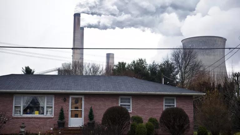
How to Start Saving the Planet in 100 Days: the Joe Biden Edition

When you sign up, you’ll become a member of NRDC’s Activist Network. We will keep you informed with the latest alerts and progress reports.

Confronting the Nation's Water Problems: The Role of Research (2004)

Chapter: 5 data collection and monitoring, 5 data collection and monitoring.

The long-term monitoring of hydrologic systems and archiving of the resulting data are activities that are inseparable from the water resources research enterprise of the nation. Data are essential for understanding physicochemical and biological processes and, in most cases, provide the basis for predictive modeling. Examples of water resources and other relevant data that are collected through a variety of measurement devices and networks are:

hydrologic storages and fluxes such as soil moisture, snow pack depth, precipitation, streamflow, hydraulic head, recharge, and evapotranspiration

land-ocean-atmosphere energy fluxes

water, land, and air quality measures, including physical, chemical, biological, and ecological elements

water and energy demand, consumptive use, and return flows

terrain elevation and land use, and lake, stream, and river geometry

Data collection is the means by which these types of data are acquired for multiple uses, including for flood warnings and other health and safety monitoring activities, weather prediction, engineering design, commercial and industrial applications, and scientific research. Monitoring is data collection with the more targeted purpose of detecting and drawing attention to changes in selected measures, particularly extreme changes. Monitoring data have multiple applications. They may serve as indicators of health and safety risks, as trip wires for policy changes, or as the basis for research on variability and trends in hydrologic and related phenomena.

The full dimensions of the challenges and opportunities associated with data collection and management for the hydrologic sciences have become evident in recent years. These issues are especially important for federal agencies because these agencies are instrumental in developing new monitoring approaches, in validating their efficacy through field studies, and in managing nationwide monitoring networks over long periods.

This chapter is not a comprehensive assessment of water resources data collection activities. Rather, it is intended to highlight the importance of data collection and its role in stimulating and facilitating water resources research. Thus, it relies upon a few specific examples from certain federal agencies. As a consequence, not all data collection activities relevant to water resources research are included (e.g., active disease surveillance and monitoring of land use are not discussed), nor are all federal and state agencies that support or actively conduct monitoring mentioned.

CHALLENGES IN MONITORING

There are important challenges facing federal agencies that collect and manage hydrologic data. One of these challenges is related intrinsically to the types of problems for which hydrologic data are being used. For example, the analysis of problems related to floods and droughts requires specific information about extreme events, which can be developed only after conducting decades or even centuries of precipitation and streamflow monitoring across a variety of different climatic and hydrologic settings. Similarly, an assessment of the impact of global climate change on groundwater and surface water resources will require basic monitoring systems capable of providing data for time periods of centuries. With other problems, like nonpoint source contamination of streams resulting from runoff laden with nitrate, pesticides, and sediment, hourly data may be required because of the close association of stream contamination with the timing of storms and resulting runoff processes. In this case, the greater challenge is encompassing all relevant spatial scales, because the local variability in contaminant loading is related to changes in land use and farming practices. In general, the broad spectrum of present and future scientific water problems nationwide requires monitoring systems that function reliably over both large and small time and space scales.

Unfortunately, as described in detail in later sections, observational networks to measure various water characteristics have been in decline during the last 30 years because of political and fiscal instabilities (e.g., NRC, 1991; Entekhabi et al., 1999). The following sections provide a detailed discussion of how several national monitoring networks have fared over time. The funding situation for monitoring networks is remarkably similar to that for research on improving data collection activities (Category VII), which Chapter 4 showed as having declined to a level that is only a fourth of its value in the mid 1970s. These facts point to

the need for increased funding for in situ data networks as a necessary complement to water resources research activities.

Unquestionably, the complexity of monitoring has increased dramatically as researchers have begun to sort out the interactions among physical, chemical, and biological processes in water (Pfirman and AC-ERE, 2003). Before 1960, hydrologic monitoring in the U.S. Geological Survey (USGS) emphasized streamflows, sediment transport, and groundwater levels. As problems of contamination became more evident, monitoring expanded to examine basic water quality variables. Now, monitoring encompasses a variety of anthropogenic compounds in water and sediment, aquatic organisms, and other biological characteristics. In just the past few years, advances in analytical techniques and the discovery of new, ecologically significant families of contaminants have made the need for comprehensive monitoring of aquatic systems even more evident.

Federal agencies are under significant pressure to respond to the increasing need for chemical and biological monitoring of aquatic systems. The creation of the National Water Quality Assessment (NAWQA) program of the USGS high-lights the emerging importance of this type of monitoring, as well as its complexity and potential costs. Yet, even this large program is only a first step in providing the information necessary to support federal regulations related to water quality (e.g., the Total Maximum Daily Load program), to support restoration of aquatic ecosystems impacted by agriculture (e.g., the Neuse River basin), and to promote the sustainability of water resources (e.g., the Rio Grande). The development of the kind of enhanced chemical and biological monitoring that will be needed to address such issues remains a challenge.

Complexity in monitoring also arises because of the scales at which problems are now manifested. For example, the study of hypoxia in the northern Gulf of Mexico is inexorably linked to the Mississippi–Atchafalaya River Basin, which drains an area of 3.2 million square miles (NSTC, 2000). New, scale-appropriate techniques will be required to examine hydrologic conditions across watersheds of subcontinental proportions. Unfortunately, such large-scale monitoring approaches are in their infancy and are not sufficiently developed to meet even immediate needs for some classes of problems. As will be discussed shortly, this challenge to provide new kinds of data is also an opportunity for innovative research related to space-borne and sensor technologies.

The increasing variety and quantity of information coming from monitoring systems have created new problems of data warehousing and dissemination. Federal and state agencies over time have developed important databases (e.g., the Environmental Protection Agency’s [EPA] STORET and USGS’ NWIS) that are an increasingly useful way to identify problems and research needs. However, as a consequence of historical agency responsibilities and/or lack of national funding, federal water resources data are spread among different federal and state agencies with broadly different capabilities for supporting user needs and with different resources for making important legacy data available to researchers. Taylor and

Alley (2001) point out that many state agencies have backlogs of data waiting to be summarized in electronic databases. (Indeed, one agency representative reported that summer students were used to develop web sites that can disseminate valuable historical data from research watersheds.) There is little consistency in federal and state programs for recovering the costs of monitoring. Some monitoring data (e.g., some stream discharge data) are freely available, while in other cases (e.g., Landsat), Congress has mandated cost recovery for the data, which makes using such data expensive in research and may limit their creative use.

An important aspect of improving hydrologic data collection is to take into account the uncertainties associated with both data collection methods and the design of data collection networks. Hydrologic forecasting relies heavily on measurements of multiple hydrologic variables taken over long periods of time, particularly because low-frequency but high-magnitude events can have near-irreversible effects on water supply. As monitoring networks decrease in size and density, uncertainty increases. Methods of rescuing and augmenting the available data are needed to reduce the uncertainty of predictions. Similarly, methods of validating and estimating the uncertainty of remotely sensed data are needed, as these sources of data are becoming increasingly important in hydrologic analyses.

OPPORTUNITIES IN MONITORING

Hydrologists working in the United States can now take advantage of new monitoring data and new technical approaches for monitoring hydrologic processes. Important advances for the diagnosis and prediction of hydrologic processes have come from remote sensing using products derived from observations that span a wide range of the electromagnetic spectrum (e.g., visible, infrared, microwave) (Owe et al., 2001). For example, Landsat satellites have provided a significant record of land-cover conditions on the earth’s surface and an ability to monitor land-use changes (e.g., Running et al., 1994), and they can measure water clarity and chlorophyll in lakes ( www.water.umn.edu ). Remote sensing has also been shown to provide significant information about hydrologic extremes, such as drought, and to have the potential to enhance our ability to forecast these events (e.g., Kogan, 2002). New satellite sensors (e.g., Advanced Microwave Sounding Unit on the National Oceanic and Atmospheric Administration [NOAA] 15, 16, and 17 satellites) with the ability to penetrate cloud cover and produce land surface moisture products with temporal resolutions of hours and spatial resolutions of tens of kilometers promise to enhance our operational database that supports water supply forecasts (Ferraro et al., 2002). Chlorophyll levels in freshwater lakes now are being mapped routinely by satellite. Furthermore, high-resolution satellites are being used to map distributions of different types of aquatic plant communities in wetlands and littoral areas of lakes, and aircraft-mounted spectroradiometers are being used to map aquatic vegetation and water quality conditions (e.g., turbidity, phosphorus, and chlorophyll a ) in rivers.

Radar altimeters, like TOPEX/Poseidon and Jason-1, which have been used mostly for measuring changes in sea level, are also useful for measuring the stages of large rivers and lakes (Birkett, 1995, 1998). The laser altimeters aboard ICESat, although not particularly reliable at the present stage of development, have demonstrated the potential to measure water-surface elevations for small waterbodies on a regular basis. The Gravity Recovery and Climate Experiment (GRACE) mission provides unprecedented capabilities to assess changes in water storage over large regions (Rodell and Famiglietti, 1999, 2002). GRACE is anticipated to provide monthly measurements of total water storage anomalies with a spatial scale of longer than several hundred kilometers, and with an accuracy of a few millimeters in water-height change.

Ground-based remote sensing monitoring systems have been developed that are applicable to water resources investigations of regional water supplies. A good example is the widespread national deployment of the WSR-88D weather radar (NEXRAD). Each NEXRAD station monitors thousands of square kilometers and provides almost continuous space-time estimates of precipitation with kilometer resolution (e.g., Klazura and Imy, 1993). When properly calibrated, these systems can provide highly resolved estimates of precipitation for complex storms or for regions where coverage by conventional gages is limited (e.g., Seo et al., 2000).

Remote sensing will undoubtedly change the way that some hydrologic monitoring is carried out, although routine use of some of these technologies for water resources research is still years away. In the meantime, the use of the remotely sensed data for water resources research on regional and local scales will require validation and adjustment with legacy monitoring measurements and, for many applications, combined use with in situ measurements of longer records. For example, it is expected that detailed monitoring of chemical and biological conditions will still require sampling and laboratory analyses or in situ sensor measurements, and likely some combination of both. Fortunately, technological advances are being made in developing low-cost and reliable sensors and miniaturized in situ instruments to measure a wide variety of chemical and biological contaminants in natural waters (ASLO, 2003).

In addition to requiring validation with legacy monitoring, profitable use of remotely sensed data will require measurements of associated space-time observation uncertainty. Such efforts are required because remote sensors in many cases do not directly measure the quantity of interest, because the data they generate carry biases due to atmospheric and land surface interference, or because their penetration depth into the land surface is shallow. In addition, regional and local databases of remotely sensed data in most cases have short record lengths that are often inadequate for the study of water supply variability, including climate extremes. It should be noted that remote sensing systems for some crucial water monitoring data—for example biological metrics of water quality like

numbers and health of algae, invertebrates, fish, and aquatic and terrestrial plants—are only now being developed.

Thus, although there is much progress with respect to remote sensing systems measurement and monitoring, important in situ monitoring systems are in decline without clear plans for transitioning to new or alternative technologies. Because of the “stovepiping” within agencies, there is no overall coordination in operating monitoring systems and in determining directions of new technological initiatives.

A new paradigm for data acquisition and management is offered by the cyberinfrastructure view of information, which is a significant step for enabling the next generation of research in science and engineering. The National Science Foundation (NSF) is at the forefront of this important new initiative, which recognizes the ability of new developments in information technologies to change the way data are collected, managed, and used (Atkins et al., 2003). The term cyberinfrastructure refers to the variety of approaches (some new, some old) for the creation, dissemination, and preservation of knowledge. The NSF vision is “to use cyberinfrastructure to build more ubiquitous, comprehensive digital environments that become interactive and functionally complete for research communities in terms of people, data, information tools, and instruments” (Atkins et al., 2003). The development of these approaches is a bold step forward in the seamless integration of experimentation and data collection.

The most important implication of cyberinfrastructure for water resources is that monitoring is not simply an isolated task but is part of an integrated information strategy that more directly connects researchers with data and the actual process of measurements. If properly executed, this strategy has the potential to create a more uniform technological vision among federal agencies and to reduce redundancies in data handling among federal agencies. In other words, there are opportunities for government agencies concerned with monitoring to develop a systemic approach to handling the explosion of new data and the operation and maintenance of monitoring systems. Federal agencies are relatively independent in their approaches and solutions to issues of monitoring and data management.

STATUS OF KEY MONITORING PROGRAMS

Addressing water resources concerns in the future will require increasingly sophisticated monitoring data. Streamflow data, for example, are necessary to (1) support important public policy decisions concerning towns located in the floodplains of rivers like the Mississippi, (2) engineer structures to limit flood damages from rivers like the Red River of the North, and (3) manage water resources in important western rivers like the Colorado. Chemical, biological, and sediment data are needed to evaluate the efficacy of attempts to restore water quality and ecological health in the Chesapeake Bay, the Mississippi River system, and the San Francisco Bay, which are being adversely affected by nonpoint source contamination. Global climate change is predicted to have major impacts

on rivers of the northwestern United States and the Prairie Pothole region of the northern Great Plains (NAST, 2000) and will require new monitoring networks.

The following sections provide examples of the national decline in some types of monitoring systems and the funding limitations that have stifled efforts toward new national systems in groundwater and soil-moisture monitoring. The lack of investment in hydrologic monitoring is hard to reconcile, given the societal cost and significance of problems affecting water resources now and in the future. The reasons for the decline are many and speculative. It is possible that the distributed nature of water resource problems and the long periods between extreme events have obscured the need for monitoring systems (i.e., it is too early to see the negative impacts of the cuts in monitoring). Alternatively, it may be that the consequences of dismantling or substantially reducing monitoring systems have been small to date because accumulated science and engineering knowledge has been able to cope to some extent with the uncertainties of reduced observations. Another possibility that might account for the observed decline is that there are likely fewer and less visible investments in large water resources structures (e.g., dams, reservoirs, canals, and reclamation projects) that might require data.

The responsibilities for collecting, maintaining, and distributing hydrologic data remain with federal agencies, and this situation is not likely to change, given the nature of water resources data collection as a public good (see Chapter 1 ). The dilemma of the federal agencies is how to simultaneously maintain legacy monitoring systems, respond to escalating needs for expanded monitoring of all kinds, and take advantage of new opportunities in infrastructure development for measurement and data management.

The USGS has been collecting streamflow information since 1889 and today operates a national network of about 7,200 stream gages. The information provided by the network is used for many purposes, including water resource planning, daily water management, flood prediction and hazard estimation, water quality assessment and management, aquatic habitat assessment and mitigation, engineering design, recreation safety, and scientific research. Funding for the network comes from the USGS and over 800 other federal, state, and local agencies. This unique arrangement helps ensure streamflow information relevant to local needs; however, it also means that the USGS does not have complete control over the network, including the number or location of the individual stream gages that constitute the network.

Stream gages with long periods of record are of great importance for estimating hydrologic extremes (floods and droughts) and for resource planning. These gages are crucial to describing and understanding the effects of climate, land-use, and water-use changes on the hydrologic system. However, maintaining stream gages with a long period of record is not always a priority of many partner agen-

cies. As a consequence, there has been an alarming loss of stream gages with 30 or more years of record over the last three decades, even though the total number of stream gages in the network has remained relatively constant (Norris, 2000). In the period 1990–2001, 690 stream gages with 30 or more years of record were discontinued; nearly 170 of those were discontinued in 1995 alone.

The USGS has described the instability of the national stream gaging network as being related to the current dominant funding process of stream gages and has proposed plans to modernize, stabilize, and fill critical gaps in the network (USGS, 1999; Hirsch and Norris, 2001). This plan, called the National Streamflow Information Program (NSIP), would provide for a stable nationwide backbone stream gage network that would be fully funded by the USGS to maintain for future generations the important long-term streamflow information at critical locations. Stream gages required for local needs would supplement this backbone network and would remain funded through the Cooperative Water Program. In addition to providing a stable component to the national stream gaging network, NSIP would also enhance the value of all streamflow information obtained by the USGS by improving and modernizing data delivery, obtaining more information during hydrologic extremes than is currently obtained, analyzing streamflow information to provide insights on key characteristics (e.g., long-term trends and their relationship to natural and anthropogenic features within watersheds), and conducting research and development aimed at improving instruments and methods in order to provide more accurate, more timely, and less expensive streamflow information in the future. According to NRC (2004), the NSIP program adequately takes into account both the spatial distribution (in terms of value and need) of gages and the use of modeling to provide information about ungaged locations. This is an ambitious program that would require a considerable long-term financial commitment from Congress and the executive branch. So far, only minor additional funding has been appropriated for this program.

Groundwater Levels

Water-level measurements from observation wells are the principal source of information about the effects of hydrologic stresses on groundwater systems. In recent years, the USGS and many state and local agencies have experienced difficulties in maintaining long-term water-level monitoring programs because of limitations in funding and human resources. A poll of USGS district offices and 62 state and local water management or regulatory agencies about the design, operation, and history of long-term observation wells in their respective states indicated that there are about 42,000 observation wells in the United States with five years (a relatively short period) or more of water-level record data (Taylor and Alley, 2001). About a quarter of those are monitored under the USGS Cooperative Water Program. The level of effort in collecting long-term water-level data varies greatly from state to state, and many of the long-term monitoring

wells are clustered in certain areas. Although difficult to track, the number of long-term observation wells appears to be declining. For example, the number of long-term observation wells monitored by USGS has declined by about half from the 1980s to today (Alley and Taylor, 2001).

Groundwater-level data become increasingly valuable with length and continuity of record. Ease of access to the data and their timeliness also are valuable, especially during periods of stress such as droughts. Although real-time surface water data have been available through the Internet for nearly a decade, the availability of real-time groundwater data is relatively new within the USGS. Between the years 2000 and 2003, real-time data for wells available through the Internet went from fewer than 300 wells (mostly in south Florida) to nearly 700 wells. Real-time data applications allow effective aquifer management, produce high-quality data, and can be cost-effective. As the availability and reliability of real-time groundwater data increase, so will their value to scientists and the public.

Despite the existence of thousands of observation wells across the nation, most groundwater-level data collection is funded to address state and local issues. Yet, there is evidence that more groundwater problems are becoming regional or national in scale, as exemplified by interstate conflicts over groundwater sources becoming salinized or overdrawn. A case in point is the High Plains aquifer, which encompasses eight states in the central United States. In parts of Kansas, New Mexico, Oklahoma, and Texas, current groundwater withdrawals, primarily used for irrigation, are unsustainable because the natural recharge is low, resulting in a dramatic decline in groundwater levels (Alley et al., 1999). Given the increasing reliance on groundwater sources (Glennon, 2002), it is important to understand trends in groundwater levels and quality over large regions. Unfortunately, there is no comprehensive national groundwater-level network with uniform coverage of major aquifers, climate zones, or land uses. In fact, data on groundwater levels and rates of change are “not adequate for national reporting” according to the report The State of the Nation’s Ecosystems (H. John Heinz III Center, 2002). Data are not collected using standardized approaches at similar spatial or temporal scales, and the long-term viability of the data collection efforts is uncertain. Ideally, a comprehensive groundwater-level network is needed to assess groundwater-level changes, the data from which should be easily accessible in real time.

Soil Moisture

It has been long recognized that soil moisture in the first one or two meters below the ground surface regulates land-surface energy and moisture exchanges with the atmosphere and plays a key role in flood and drought genesis and maintenance (e.g., Huang et al., 1996; Eastman et al., 1998). Soil moisture deficit partially regulates plant transpiration and, consequently, constitutes a diagnostic

variable for irrigation design (e.g., Dagan and Bresler, 1988). High extremes of soil moisture are associated with high potential for flooding and hazardous conditions. As the “state variable” of the vadose zone, soil moisture plays a key role in surface–subsurface water exchanges. Although the importance of soil moisture for hydrologic science and applications cannot be overemphasized, there are few long-term and large-scale measurement programs for soil moisture that provide in situ profile data suitable for hydroclimatic analysis and design in the United States (e.g., Hollinger and Isard, 1994; Georgakakos and Baumer, 1996) and abroad (e.g., Vinnikov and Yeserkepova, 1991). Active and passive microwave data from polar orbiting satellites or reconnaissance airplanes do provide estimates of surface soil moisture with continuous spatial coverage. However, they are limited in that they only measure soil moisture within the first few centimeters of the soil surface, and they are reliable only when vegetation cover is sparse or absent (e.g., Ulaby et al., 1996; Jackson and Le Vine, 1996).

This lack of long-term soil moisture data over vast areas of the United States affects how well soil moisture is incorporated into hydrologic models for watersheds or large regions. At the present time, models must use estimates derived from secondary sources of information or from other models, rendering predictions pertaining to ecosystem behavior or surface water–groundwater interactions subject to significant uncertainty. Even a few long-term monitoring networks of soil moisture would substantially decrease the uncertainty in predicting processes that critically depend on soil moisture levels (like flow, water chemistry, and plant response). In a similar vein, the uncertainty of predictive models for managing water supply in western streams reflects the density of streamflow and rainfall monitoring networks, because the amount and the quality of data in areas characterized by high spatial variability in precipitation determine how reliable and precise such models can be.

The development of a national soil moisture monitoring network is an essential element to conducting successful research on the physical, chemical, and biological processes in the surface layer of the continental United States. The U.S. Department of Agriculture (USDA) Natural Resources Conservation Service has established a coordinated national network of in situ measurements of soil moisture and soil temperature in support of agricultural needs (Soil Climate Analysis Network or SCAN). Although this is a step in the right direction, significant expansion of the network into nonagricultural areas together with a long-term commitment for high quality data are necessary for water resources analysis on climatic and regional scales. Furthermore, modeling and observational studies have shown substantial soil moisture variability over a range of scales (e.g., Rodriguez-Iturbe et al., 1995; Guetter and Georgakakos, 1996; Vinnikov et al., 1996; Lenters et al., 2000), and the development of a monitoring plan for soil moisture on the basis of both remotely sensed and on-site data is a requisite research endeavor that should account for such variability.

Water Quality

Water quality monitoring has seen declining trends in funding similar to those for streamflow and groundwater level monitoring. Both the EPA, through its Environmental Monitoring and Assessment Program (EMAP), and the states, through their delegated authority from EPA for the Clean Water Act, conduct some water quality monitoring. Unfortunately, efforts are inconsistent from state to state and are often inadequate, and some are in decline. Recent reports (e.g., GAO, 2000; NRC, 2002a; Mehan, 2004) cite the need for consistent ambient water quality data for purposes of Clean Water Act compliance. The current shortfalls and future needs are illustrated below using USGS water quality programs as examples.

For some areas, USGS data are relied upon to establish trends in water quality over time and to compare conditions across local jurisdictional boundaries. Unfortunately, water quality monitoring networks within USGS have not received additional funding since their inception and thus have been declining simply due to the impacts of inflation. USGS surface water quality networks include the Hydrologic Benchmark Network (HBN), operating since 1964, and the National Stream Quality Accounting Network (NASQAN), operating since 1973. HBN monitors small watersheds in areas relatively free from human impacts, from water diversions, and from water impoundments, providing important baseline data for understanding water quality impairments and needed improvements. When it first began in 1964, HBN water quality sampling was quarterly to monthly depending on location, but since 1997 there has been no water quality sampling at the 52 watersheds (Mast and Turk, 1999). Beginning in 2003, limited sampling resumed at 15 of the remaining 36 watersheds. 1

NASQAN measures water quality in the nation’s largest river systems, and it also includes many coastal drainages. At the program’s operational peak (in 1976), more than 500 locations were sampled either monthly or six times a year for major ions, nutrients, trace metals, indicator bacteria, and periphyton. Now, only 33 sites remain, with sampling at a frequency adequate for annual flux estimates and with new capabilities for sampling some pesticides. These networks now provide a fraction of the data they once produced (though some prior components may be handled by the NAWQA program—see below).

Assessing water quality, both for trends over time and for causative factors, is growing in importance for water resource management. The NAWQA program provides data and information on the most important (defined by water use for municipal supply or irrigated agriculture) river basins and aquifer systems (study units). NAWQA comprehensively samples surface water and groundwater for physical and chemical variables, and it produces data on aquatic communities of

fish, insects, and algae. Originally NAWQA was designed for sampling 59 study units, but by 2001 only 51 were sampled, and now because of funding constraints only 42 study units continue to operate.

Within NAWQA, many sampling activities have been curtailed. For example, between 1993 and 2001, more than 600 fixed-station surface water sites were sampled, but now only about 150 sites continue to operate. These sites provide the only continuous water quality trend sampling. Although thousands of bed sediment and tissue data were collected from streams in the first years of sampling, most of those sampling efforts cannot be repeated. Groundwater sampling between 1993 and 2001 included more than 6,500 wells. There are not adequate resources to sample those sites repeatedly for trends, and only 2,400 wells are being resampled in urban, agriculture, and large aquifer networks, reducing substantially the density of the sampling network. Although the numbers of wells may seem large, the trend network provides insight at an average of less than 60 wells per study unit (the median study unit area is 21,000 sq. mi.). The recent National Research Council (NRC) report (NRC, 2002a) states that NAWQA cannot decrease its number of study units further and still provide the national scope of data called for by Congress.

Monitoring activities related to sediment are particularly crucial because it is the most widespread pollutant in U.S. rivers (EPA, 2002). The USGS is the principal source of fluvial-sediment data, providing daily suspended-sediment discharge data at about 105 sites (sediment stations) in 2002. These data serve traditional uses that include design and management of reservoirs and in-stream hydraulic structures and dredging. In the last two decades, information needs have expanded to include those related to contaminated sediment management, dam decommissioning and removal, environmental quality, stream restoration, geomorphic classification and assessments, physical–biotic interactions, the global carbon budget, and regulatory requirements of the Clean Water Act including the EPA’s Total Maximum Daily Load program.

An increasing need for fluvial-sediment data has coincided with a two-thirds decline in the number of USGS sediment stations from the peak of 360 in 1982 (Gray, 2002) to about 105 sites now. Among the factors cited for the decline in the number of USGS daily sediment stations was the need for less expensive and more accurate fluvial-sediment data collected using safer, less manually intensive techniques. Any decrease in sediment monitoring should be of particular concern given that the physical, chemical, and biological sediment damages in North America alone were estimated at $16 billion in 1998 (Osterkamp et al., 1998). In its review of the NAWQA program, the NRC noted the serious need to improve sediment monitoring (NRC, 2002a).

Box 5-1 discusses how the lack of reliable water quality monitoring data has hampered efforts to sensibly plan for development in New Jersey and comply with state laws. It exemplifies not only shortages in groundwater quality data, but also in flow data.

Estimating the demands for water and amounts withdrawn from various surface-water and groundwater sources is of critical importance to water resources management. Since 1950, the USGS has compiled and disseminated estimates of water use for the nation at five-year intervals. Most of the data are collected, however, not by the USGS but by the individual states to support their water-use permitting and registration programs. Although matching funds for the analysis and aggregation of water use data are often available through the USGS Cooperative Water Program, some states make little effort in this area. Thus, the quality of water use data varies considerably from state to state. Unfortunately, because of funding limitations, the USGS had to reduce the scope of reporting on a nationwide basis in 2000 for several categories of water use. Reductions in national scope included (1) eliminating estimates of commercial use and hydroelectric power (which is counter to recommendations in the Envisioning report [NRC, 2001]), (2) providing information for mining, livestock, and aquaculture only for large-use states, (3) eliminating estimates of consumptive use and public deliveries, and (4) compilation at the county, but not watershed, level.

In a recently completed NRC review of the USGS National Water Use Information Program (NWUIP) (NRC, 2002b), basic questions about the nature of water use, the water use information needed in the United States, and the USGS role in generating and disseminating that information were considered. Major recommendations contained in the NRC report include the following:

The NWUIP should be elevated to a water use science program (rather than a water use accounting program), emphasizing applied research and tech-

niques development in the statistical estimation of water use and the determinants and impacts of water-using behavior.

To better support water use science, the USGS should build on existing data collection efforts to systematically integrate datasets, including those maintained by other federal and state agencies, into datasets already maintained by the NWUIP.

The USGS should systematically compare water use estimation methods to identify the techniques best suited to the requirements and limitations of the NWUIP. One goal of this comparison should be to determine the standard error for every water use estimate.

The USGS should focus on the scientific integration of water use, water flow, and water quality to expand knowledge and generate policy-relevant information about human impacts on both water and ecological resources.

The USGS should seek support from Congress for dedicated funding of a national component of the recommended water use science program to supplement the existing funding in the Cooperative Water Program.

The preceding section discussed some of the important data collection networks relevant to water resources research, but the discussion was not intended to be exhaustive. For example, both public health data collection (e.g., active disease surveillance) and monitoring of climate variables like precipitation were not discussed. This should not be interpreted as implying that they are less important types of data. Indeed, Box 5-2 discusses how federally funded monitoring for climate indices is routinely used to manage water resources in the Florida Everglades.

CONCLUSIONS AND RECOMMENDATIONS

Monitoring efforts are inseparable from the research efforts described in other chapters of this report. Furthermore, they are critical to addressing water resources problems related to floods and droughts, agricultural sustainability, global climate change, and other high priorities for water resources research (as expressed in Chapter 3 ). Indeed, the continuing need for high-quality, long-term in situ data was the only water resources-related issue expressed unanimously by 13 state government representatives who addressed the committee in January 2003 (see Appendix D ).

The challenges to the monitoring of water resources are formidable and include a sizable increase in the number of features to be monitored, as the variety, scope, and complexity of problems expand, especially with respect to biological issues; a major expansion in the range of time/space scales that must be addressed by data collection and monitoring as new, major problems develop; and difficulties in making the increasingly large amounts of data available quickly and efficiently. The following conclusions and recommendations address the need to match these challenges, as well as emerging water resources problems, with new investments for basic data collection and monitoring.

Key legacy monitoring systems in areas of streamflow, groundwater, sediment transport, water quality, and water use have been in substantial decline and in some cases have been nearly eliminated. These systems provide data necessary for both research (i.e., advancing fundamental knowledge) and practical applications (e.g., for designing the infrastructure required to cope with hydrologic extremes). Despite repeated calls for protecting and expanding monitoring systems relevant to water resources, these trends continue for a variety of reasons.

The consequences of the present policy of neglect associated with water resources monitoring will not necessarily remain small. New hydrologic problems are emerging that are of continental or near continental proportions. The most obvious are the likely impact of global climate change on water resources; hypoxia in the Gulf of Mexico, related to nutrient loading from the Mississippi River; and the questionable sustainability of the water supply for western and southern regions given population increases and recent interest in restoring aquatic ecosystems (e.g., the Florida Everglades and the Mississippi River basin). The scale and the complexity of these problems are the main arguments for improvements to the in situ data collection networks for surface waters and groundwater and for water demand by sector. It is reasonable to expect that improving the availability of data, as well as improving the types and quality of data collected, should reduce the costs for many water resources projects.

Notwithstanding the overall decline in legacy monitoring systems, there are some positive developments that bear on hydrologic monitoring. For example, the NEXRAD system provides unprecedented spatial resolution of rainfall distribution. Efforts have continued to support environmental earth-surface observations with new generations of satellites. Other NASA research missions (e.g., IceSat, TOPEX/Poseidon, GRACE) give positive early indications of their potential as monitoring tools for hydrologic systems. Although these new satellite-based measuring systems have important applications to hydrologic research, they are not yet ready to replace legacy monitoring systems. Moreover, for chemical, biological, and groundwater monitoring, in particular, new in situ and remote

sensing technologies capable of replacing wells or field sample collections are still in development.

Increases in strategic investments for monitoring are necessary to avoid or at least reduce costs attendant with future water resource or health crises . Investments are required but are not by themselves sufficient to ensure that the data necessary to attack 21st century problems will be available to researchers and policy makers alike. Federal agencies need to adopt a research perspective toward monitoring and data collection that better integrates monitoring with the research efforts described in other chapters of this report. There is also a strong need for cooperation among agencies concerned with collecting, storing, and managing hydrologic data, particularly from research watersheds and legacy monitoring systems. The NSF cyberinfrastructure initiative is an example of a visionary approach for creating comprehensive digital environments linking people and data. It is recommended that an interagency task force concerned with information technology and data management be established and that it develop a non-NSF federal cyberinfrastructure community.

Alley, W. M., T. E. Reilly, and O. L. Franke. 1999. Sustainability of ground-water resources. U.S. Geological Survey Circular 1186.

Alley, W. M., and C. J. Taylor. 2001. The value of long-term ground water level monitoring. Ground Water 39:801.

American Society of Limnology and Oceanography (ASLO). 2003. Emerging Research Issues for Limnology: the Study of Inland Waters. Waco, TX: ASLO.

Atkins, D. E., K. K. Droegemeir, S. I. Feldman, H. Garcia-Molina, M. L. Klein, D. G. Messerschmitt, P. Messina, J. P. Ostriker, and M. H. Wright. 2003. Revolutionizing Science and Engineering through Cyberinfrastructure. Washington, DC: National Science Foundation.

Birkett, C. M. 1995. The contribution of TOPEX/POSEIDON to the global monitoring of climatically sensitive lakes. JGR–Oceans 100 (C12):25,179–25,204.

Birkett, C. M. 1998. Contribution of the TOPEX NASA radar altimeter to the global monitoring of large rivers and lakes. Water Resources Research 34(5):1223–1239.

Dagan, G., and E. Bresler. 1988. Variability of an irrigated crop and its causes: 3—numerical simulation and field results. Water Resources Research 24(3):395–401.

Eastman, J. L., R. A. Pielke, and D. J. McDonald. 1998. Calibration of soil moisture for large-eddy simulations over the FIFE area. J. Atmospheric Sciences 55:1–10.

Entekhabi, D., G. R. Asrar, A. K. Betts, K. J. Beven, R. L. Bras, C. J. Duffy, T. Dunne, R. D. Koster, D. P. Lettenmaier, D. B. McLaughlin, W. J. Shuttleworth, M. T. van Genuchten, M. Y. Wei, and E. F. Wood. 1999. An agenda for land surface hydrology research and a call for the second international hydrological decade. Bull. Amer. Meteor. Soc. 80:2043–2058.

Environmental Protection Agency (EPA). 2002. National Water Quality Inventory—2000 report: EPA–841–R–02–001. Washington, DC: EPA.

Ferraro, R., F. Weng, N. Grody, I. Guch, C. Dean, C. Kongoli, H. Meng, P. Pellegrino, and L. Zhao. 2002. NOAA satellite–derived hydrological products prove their worth. EOS 83(29):429–438.

General Accounting Office (GAO). 2000. Key EPA and State Decisions Limited by Inconsistent and Incomplete Data. General Accounting Office RCED–00–54. 73 p. Washington, DC: GAO.

Georgakakos, K. P., and O. W. Baumer. 1996. Measurement and utilization of on-site soil moisture data. Journal of Hydrology 184:131–152.

Glennon, R. 2002. Water Follies: Groundwater Pumping and the Fate of America’s Fresh Waters. Washington, DC: Island Press.

Gray, J. R. 2002. The need for sediment surrogate technologies to monitor fluvial-sediment transport. Proceedings of the Turbidity and Other Sediment Surrogates Workshop, April 30–May 2, 2002, Reno, Nevada. http://water.usgs.gov/osw/techniques/TSS/listofabstracts.htm .

Guetter, A. K., and K. P. Georgakakos. 1996. Large-scale properties of simulated soil water variability. J. Geophysical Research—Atmospheres 101(D3):7175–7183.

H. John Heinz III Center for Science, Economics and the Environment. 2002. The State of the Nation’s Ecosystems: Measuring the Lands, Waters, and Living Resources of the United States. Cambridge, UK: Cambridge University Press.

Hirsch, R. M., and J. M. Norris. 2001. National Streamflow Information Program: Implementation Plan and Progress Report. USGS Fact Sheet FS–048–01.

Hollinger, S. E., and S. A. Isard. 1994. A soil moisture climatology of Illinois. J. Climate 7(5):822–833.

Huang, J., H. M. Van den Dool, and K. P. Georgakakos. 1996. Analysis of model-calculated soil moisture over the United States (1931–1993) and applications to long-range temperature forecasts. J. Climate 9(6):1350–1362.

Jackson, T. J., and D. E. Le Vine. 1996. Mapping surface soil moisture using an aircraft-based passive microwave instrument: algorithm and example. J. Hydrology 184:85–99.

Klazura, G. E., and D. A. Imy. 1993. A description of the initial set of analysis products available from the NEXRAD WSR–88D System. Bulletin of the American Meteorological Society 74:1293–1312.

Kogan, F. 2002. World droughts in the new millennium from AVHRR-based vegetation health indices. EOS 83(48):557–563.

Lenters, J. D., M. T. Coe, and J. A. Foley. 2000. Surface water balance of the continental United States, 1963–1995: regional evaluation of a terrestrial biosphere model and the NCEP/NCAR reanalysis. J. Geophysical Research—Atmospheres 105(D17).

Mast, M. A., and J. T. Turk. 1999. Environmental Characteristics and Water Quality of Hydrologic-Benchmark Network Stations in the Eastern United States 1963–95. U.S. Geological Survey Circular 1173–A. 158 p.

Mehan, T. 2004. Better monitoring for better water management. Water Environmental Research 76(1): 3–4.

National Assessment Synthesis Team (NAST). 2000. Climate change impacts on the United States: The potential consequences of climate variability and change. Washington, DC: U.S. Global Change Research Program.

National Research Council (NRC). 1991. Opportunities in the Hydrologic Sciences. Washington, DC: National Academy Press.

National Research Council (NRC). 2001. Envisioning the Agenda for Water Resources Research in the Twenty-first Century. Washington, DC: National Academy Press.

National Research Council (NRC). 2002a. Opportunities to Improve the U.S. Geological Survey National Water Quality Assessment Program. Washington, DC: National Academy Press.

National Research Council (NRC). 2002b. Estimating Water Use in the United States—A New Paradigm for the National Water-Use Information Program. Washington, DC: National Academy Press.

National Research Council (NRC). 2004. Assessing the National Streamflow Information Program. Washington, DC: The National Academies Press.

National Science and Technology Council (NSTC). 2000. 2000 Annual Report. Washington, DC: NSTC.

Norris, J. M. 2000. The value of long-term streamflow records. Water Resources Impact 2(4):11.

Osterkamp, W. R., P. Heilman, and L. J. Lane. 1998. Economic considerations of a continental sediment-monitoring program. International Journal of Sediment Research 13(4):12–24.

Owe, M., K. Brubaker, J. Ritchie, and A. Rango (eds.). 2001. Remote Sensing and Hydrology 2000. IAHS Publication No. 267. Wallingford, UK: IAHS Press.

Pfirman, S., and the AC–ERE. 2003. Complex Environmental Systems: Synthesis for Earth, Life, and Society in the 21st Century: A Report Summarizing a 10–Year Outlook in Environmental Research and Education for the National Science Foundation. Washington, DC: National Science Foundation.

Rodell, M., and J. Familglietti. 1999. Detectability of variations in continental water storage from satellite observations of the time dependent gravity field. Water Resources Research 35:2705–2723.

Rodell, M., and J. Familglietti. 2002. The potential for satellite-based monitoring of groundwater storage changes using GRACE: the High Plains aquifer, Central U.S. J. Hydrol. 263(1–4):245–256.

Rodriguez-Iturbe, I., G. K. Vogel, R. Rigon, D. Entekhabi, and A. Rinaldo. 1995. On the spatial organization of soil moisture. Geophysical Research Letters 22(20):2757–2760.

Running, S. W., T. R. Loveland, and L. L. Pierce. 1994. A vegetation classification logic based on remote sensing for use in global biogeochemical models. Ambio 23:77–81.

Seo, D.-J., J. Breidenbach, R. Fulton, D. Miller, and T. O’Bannon. 2000. Real-time adjustment of range-dependent biases in WSR-88D rainfall estimates due to nonuniform vertical profile of reflectivity. Journal of Hydrometeorology 1(3):222–240.

Taylor, C. J., and W. M. Alley. 2001. Ground-Water-Level Monitoring and the Importance of Long-Term Water-Level Data. U.S. Geological Survey Circular 1217.

Ulaby, F. T., P. C. Dubois, and J. van Zyl. 1996. Radar mapping of surface soil moisture. J. Hydrology 184:57–84.

U.S. Geological Survey (USGS). 1999. Streamflow Information for the Next Century: A Plan for the National Streamflow Information Program of the U.S. Geological Survey. USGS Open-File Report 99–456.

Vinnikov, K. Y., and I. B. Yeserkepova. 1991. Soil moisture, empirical data and model results. J. Climate 4:66–79.

Vinnikov, K. Y., A. Robock, N. A. Speranskaya, and C. A. Schlosser. 1996. Scales of temporal and spatial variability of midlatitude soil moisture. J. Geophysical Research—Atmospheres 101(D3):7163–7174.

In order to confront the increasingly severe water problems faced by all parts of the country, the United States needs to make a new commitment to research on water resources. A new mechanism is needed to coordinate water research currently fragmented among nearly 20 federal agencies. Given the competition for water among farmers, communities, aquatic ecosystems and other users—as well as emerging challenges such as climate change and the threat of waterborne diseases— Confronting the Nation's Water Problems concludes that an additional $70 million in federal funding should go annually to water research. Funding should go specifically to the areas of water demand and use, water supply augmentation, and other institutional research topics. The book notes that overall federal funding for water research has been stagnant in real terms for the past 30 years and that the portion dedicated to research on water use and social science topics has declined considerably.

READ FREE ONLINE

Welcome to OpenBook!

You're looking at OpenBook, NAP.edu's online reading room since 1999. Based on feedback from you, our users, we've made some improvements that make it easier than ever to read thousands of publications on our website.

Do you want to take a quick tour of the OpenBook's features?

Show this book's table of contents , where you can jump to any chapter by name.

...or use these buttons to go back to the previous chapter or skip to the next one.

Jump up to the previous page or down to the next one. Also, you can type in a page number and press Enter to go directly to that page in the book.

Switch between the Original Pages , where you can read the report as it appeared in print, and Text Pages for the web version, where you can highlight and search the text.

To search the entire text of this book, type in your search term here and press Enter .

Share a link to this book page on your preferred social network or via email.

View our suggested citation for this chapter.

Ready to take your reading offline? Click here to buy this book in print or download it as a free PDF, if available.

Get Email Updates

Do you enjoy reading reports from the Academies online for free ? Sign up for email notifications and we'll let you know about new publications in your areas of interest when they're released.

Earth observation vital in monitoring wetland waters

Celebrated annually on 2 February, World Wetlands Day aims to raise global awareness about the importance of wetlands for our planet. This year’s theme shines a light on wetlands as a source of freshwater and encourages actions to restore them. From their vantage point of 800 km high, Earth-observing satellites provide data and imagery on wetlands that can be used to monitor and manage these precious resources sustainably.

Natural wetlands are some of the most diverse and productive ecosystems and are critical for human survival. They provide many important benefits for humanity, ranging from freshwater supply, providing food and habitat, supporting biodiversity, to flood control, improving water quality and climate change mitigation.

Yet wetlands face many challenges. According to the Ramsar Convention, 64% of the world’s wetlands have disappeared since the beginning of the last century. Some wetlands have been lost or degraded as a result of pollution, overexploitation of resources and deforestation.

On 2 February 1971, 50 years ago today, the Convention on Wetlands of International Importance was signed in Ramsar, Iran. All bodies involved in implementing the convention require up-to-date data and reliable information to better understand wetland areas, complete national inventories, perform monitoring activities, carry out assessments and put appropriate management plans in practice.

Earth observation is recognised as a reliable and cost-effective technique for analysing and quantifying various aspects of wetland waters. The monitoring of inland water bodies is essential in order to characterise water bodies, identify changes or trends in water quantity and quality, and assess how these changes impact the integrity of wetland ecosystems and the services they provide.

For example, the Ogooué River in Gabon, the fourth largest river in Africa by volume of discharge and catchment, is home to important wetlands. However, the river is largely unmonitored, and the lack of observations poses a significant challenge to management efforts.

Earth observation can help bridge this gap, providing highly valuable observations to monitor the changes in river flows and their incidence on the water regimes of downstream wetlands.

ESA’s GlobWetland Africa project has demonstrated how data from both ESA’s CryoSat mission and from the Synthetic Aperture Radar Altimeter (SIRAL) instrument onboard the Copernicus Sentinel-3 mission can be assimilated in hydrological simulation models to assess the river’s water balance and analyse changes in the inflow hydrographs to selected wetlands in response to land use changes, hydropower and climate change.

Hydrographs show the rate of flow, or discharge, over time. These models are key in understanding catchment dynamics and are an essential tool to systematically evaluate the interactions between water availability, water use sectors and future climate.

In Uganda, wetlands and other water bodies cover roughly 10% of the country’s surface, and is home to Africa’s largest lake, Lake Victoria. However, many wetlands are put under pressure from drainage and are reclaimed to provide land for local communities to increase agriculture production for the rapidly growing population.

In order to map the dynamics of the water bodies and wetlands, ESA’s GlobWetland Africa project team used four years of data from the Copernicus Sentinel-1 and Sentinel-2 missions merged together in a hybrid approach to map the extent and frequencies of water and moist soils, and used as input for preparing national wetland inventories.

The images below show wetlands along the shore of Lake Victoria and Lake Wamala. Wetlands form along narrow water streams, where the groundwater level is high, and regular floods occur. The maps show that some of the wetlands have a strong seasonal component, whereas others are moist throughout the year.

Under ESA’s Earth Observation for Sustainable Development (EO4SD) initiative , data from the Copernicus Sentinel-3 mission was used to analyse water quality in Lake Titicaca – the second largest lake in South America and a designated Ramsar site. The unique and fragile ecosystem is negatively impacted by environmental degradation, caused by natural and anthropogenic causes, including sediment runoff and soil sanitisation, untreated urban and mining effluents and unstainable agriculture, fishing and aquaculture practices.

Sentinel-3 has been used to monitor the variation of suspended matter and chlorophyll concentrations in the lake thereby helping to detect trends and hot spots over time, information which is required to make timely decisions to emerging water quality problems, such as the identification of sediment plumes, harmful algae blooms and red tides.

Christian Tottrup, DHI GRAS and project leader of EO4SD on water resource management, commented, “Earth observation is a cost-effective technology for identifying the specific time, place and concentration of pollution – information which is of utmost importance to monitor large investment projects on sanitation infrastructure around the lake.”

The contribution of Earth observation was also valued on the ground. Rene Quispe Chambi, a specialist in water resource management from the National Water Authority (Autoridad Nacional de Agua or ANA) in Peru, said, “It is our objective to integrate Earth observation data into our water monitoring systems as decision makers require this type of information.”

ESA’s Marc Paganini added, “The European Copernicus programme and its Sentinels offer unprecedented opportunities for the Ramsar Contracting Parties to conduct the necessary wetland inventory, monitoring and assessment that ensure the wise use and conservation of their wetlands, which is the primary aim of the Ramsar Convention.

“The open and free data policy of the Sentinels along with their global coverage and the assurance of long-term continuity of observations, are important incentives for wetland practitioners to routinely integrate Earth observation in their work.”

Thank you for liking

You have already liked this page, you can only like it once!

Related Articles

Space key to wetland conservation

Related links.

GlobWetland Africa

Earth Observation for Sustainable Development (EO4SD) Water

Ramsar Technical Report

The use of Earth Observation for wetland inventory, assessment and monitoring

Copernicus Sentinel-1

Copernicus Sentinel-2

Copernicus Sentinel-3

Observing the Earth

Observation Of Water Pollution

Air pollution is the introduction into the atmosphere of chemicals, particulates, or biological materials that cause discomfort, disease, or death to humans, damage other living organisms such as food crops, or damage the natural environment or built environment. The atmosphere is a complex dynamic natural gaseous system that is essential to support life on planet Earth. Stratospheric ozone depletion due to air pollution has long been agonized as a threat to human health as well as to the Earth’s ecosystems.

Essay Example on Observation Of Water Pollution Project

Indoor air pollution (see Airlock) and urban air quality are listed as of the World’s Worst Toxic Pollution Problems in the 2008 Blacksmith Institute World’s Worst Polluted Places report. Air pollution control procedures are increasingly an important part of civic administration, although their goals are far from easy to achieve. It is also noticeable that although many urban concentrations of primary pollutants, for example, smoke and sulfur dioxide, are on the decline in developed countries, this is not always true in evolving countries.

Here the desire for rapid industrial growth has often lowered urban air quality. Secondary air pollutants are generally proving a more difficult problem to eliminate than primary pollutants like smoke. Solid waste Answers must be provided about what measures are being taken to resolve this problem of solid waste in our environment. * slide 1 of 13 Solid waste is a collective term used to distinguish non-biodegradable materials and discards that come from sources like: * Households * Businesses and Commercial establishments * Manufacturers or Industrial sites

Biomedical sources like hospital and clinics.

Proficient in: Environmental Science

“ KarrieWrites did such a phenomenal job on this assignment! He completed it prior to its deadline and was thorough and informative. ”

They are the trash collected by the municipal waste management units for segregation according to the process of disposal. Solid wastes are generally composed of non-biodegradable and non-comfortable biodegradable materials. The latter refer to solid wastes whose bio deterioration is not complete; in the sense that the enzymes Of microbial communities that feed on its residues cannot cause its disappearance or conversion into another compound.

Parts of liquid waste materials are also considered as solid sates, where the dredging of liquid wastes will leave solid sedimentation, to which proper waste management techniques should also be applied. * slide off What Is Pollution Caused by Solid Waste? Solid waste pollution is when the environment is filled with non- biodegradable and Nan-comfortable biodegradable wastes that are capable of emitting greenhouse gases, toxic fumes, and particulate matters as they accumulate in open landfills.

These wastes are also capable of leaching organic or chemical compositions to contaminate the ground where such wastes lay in accumulation. Solid wastes carelessly thrown in streets, highways, and alleyways can cause pollution when they are carried off by rainwater run-offs or by flood water to the Water Pollution Chemical pollution of surface water can create health risks, because such waterways are often used directly as drinking water sources or connected with shallow wells used for drinking water.

In addition, Waterways have important roles for washing and cleaning, for fishing and fish farming, and for recreation. Another major source of drinking water is groundwater, which often has low concentrations of pathogens because the water is filtered urine its transit through underground layers of sand, clay, or rocks. However, toxic chemicals such as arsenic and fluoride can be dissolved from the soil or rock layers into groundwater.

Direct contamination can also occur from badly designed hazardous waste sites or from industrial sites. In the United States in the sass, the government set in motion the Superfine Program, a major investigation and cleanup program to deal with such sites (U. S. Environmental Protection Agency 2000). Coastal pollution of seawater may give rise to health hazards because of local contamination of fish or hellish?for instance, the mercury contamination of fish in the infamous Inanimate disease outbreak in Japan in 1 956 (WHO 1976).

Seawater pollution with persistent chemicals, such as polycarbonate phenols (Pubs) and dioxins, can also be a significant health hazard even at extremely low concentrations (Yeast and others 2001). Based on my observation here in our country maybe the result of our water pollution is our waste that we throw in different place that we can see in lake, sea and etc. That causes flood by simply throwing our waste in such different place that blocks our passage of water irrigation.

Cite this page

Observation Of Water Pollution. (2019, Nov 27). Retrieved from https://paperap.com/paper-on-pollution-observation/

"Observation Of Water Pollution." PaperAp.com , 27 Nov 2019, https://paperap.com/paper-on-pollution-observation/

PaperAp.com. (2019). Observation Of Water Pollution . [Online]. Available at: https://paperap.com/paper-on-pollution-observation/ [Accessed: 11 May. 2024]

"Observation Of Water Pollution." PaperAp.com, Nov 27, 2019. Accessed May 11, 2024. https://paperap.com/paper-on-pollution-observation/

"Observation Of Water Pollution," PaperAp.com , 27-Nov-2019. [Online]. Available: https://paperap.com/paper-on-pollution-observation/. [Accessed: 11-May-2024]

PaperAp.com. (2019). Observation Of Water Pollution . [Online]. Available at: https://paperap.com/paper-on-pollution-observation/ [Accessed: 11-May-2024]

• Coping With Water Scarcity, Poor Water Quality and Inadequate Sanitation Pages: 3 (818 words)
• CH 456: Determination of Water Hardness of Filtered and Unfiltered Water Pages: 4 (1033 words)
• The Focus of the 1996 Safe Drinking Water Act Amendments to Water Conservation Pages: 4 (1107 words)
• Introduction of Water Pollution Pages: 3 (736 words)
• Water, Land and Air Pollution Pages: 1 (296 words)
• Water Pollution in Cambodia Pages: 2 (510 words)
• Air Water and Land Pollution Pages: 14 (4155 words)
• What are the cause and effects of water pollution Pages: 5 (1482 words)
• Effect Of Water Pollution Essay Pages: 2 (306 words)
• Water Pollution Research Paper Outline Pages: 2 (537 words)

News | Jobs | Press | Contact

• Recycling Academy
• OnBoard Laboratory
• Nomadic Expo
• Local Factories
• Exploration School
• Human-Centered Research
• Technologies
• Partner area

The Itinerant Observatory of Plastic Pollution

Challenged by a plastic crisis that seems to engulf us, how to stimulate others to act and engage?

A Mobile Space Dedicated To The Observation of Plastic Pollution

The Observatory is a mobile space that contains popularized scientific data, and tools for individuals to observe the surrounding plastic pollution. It will travel from town to city, across 3 continents, to share knowledge about plastic pollution with a diversity of people around the world.

An itinerant awareness-raising space to link local pollution and global impact.

The Observatory is a small mobile container carrying popularized scientific data and tools for experimentation. It will travel from town to city to encourage citizens in areas most affected by plastic pollution, to make a difference.

Participatory Science System

Provision of observation tools and samples of polluted water from all over the world, for one’s observation of the pollution of water by micro-plastics.

Life cycle of plastics

Computer graphics highlighting different stages in the plastic’s life, from the oil well to the shop shelves, to finally ending up in the Ocean.

Plastic never disappears. It is simply invisible to the naked eye.

Information on everyday single-used plastic’s durability and its very long (or even impossible) degradation in nature. Those include plastic bags thrown away as soon as they come back from the market, straws discarded once drinks are finished, or even cigarette butts consumed during only a few minutes. These will all take hundreds of years to disappear.

Dissection of An Ordinary Plastic Waste Product

Tube of toothpaste, a packet of crisps, food tray: the display of “cups” of ordinary waste, to highlight the different layers of which they are composed, and therefore their challenging recyclability.

Air, water, soil: plastic can penetrate anywhere.

Scientific information on how air, water, and soil are contaminated, as well as concerning concrete consequences for biodiversity and human health.

Share the post "The Itinerant Observatory of Plastic Pollution"

Latest News

Henderson Expedition: The World’s Most Polluted Protected Island Gets Rid of 9 Tons of Plastic Waste

After months of preparation, the Plastic Odyssey teams arrived on Henderson Island on February 12, 2024 and succeeded, thanks to innovative low-tech s...

Henderson Expedition: Plastic Odyssey Works to Clean Up the Most Polluted Sanctuary in the World

In the heart of the South Pacific lies Henderson Island, a UNESCO World Heritage Site, but sadly designated as the world's most polluted island. Its b...

Dominican Republic: The story of Manuel Ruiz: the visionary priest behind Movearte and the plastic revolution of El Dique

In Santo Domingo we met Manuel Ruiz, a priest with a big heart, but also an entrepreneur and visionary. He initiated several socio-environmental proje...

Join the community, Subscribe to the newsletter

• Skip to primary navigation
• Skip to main content
• Skip to primary sidebar

One Time Through

Parent smarter...not harder!

Water Pollution for Kids: Fun Science Activities

April 14, 2015 by Sue Lively

I was on my stomach, in the mud, hanging at a 45° angle reaching down the side of a creek bed, to a spot below me that I couldn’t see – trying to grab a dirty water bottle stuck in the muddy bank, half submerged in water…all for my 3 1/2 year old environmentalist son.

How did I find myself here you might ask?

Well – I guess it has something to do with all the clean water activities we’ve been doing at home lately. We have been investigating water pollution, where clean water comes from, and how it gets cleaned at water treatment plants!

Today, I’m going to share with you some of the fun water pollution activities we’ve been doing at my house. You might want to try these too with your kids!

Amazon Affiliate links included in this post. See our Disclosure for full details. 

My son first became aware of the problem of water pollution when I created a hands-on polluted ocean sensory bin for him last year.

After looking at pictures of the  Great Pacific Garbage Patch  together, Onetime spent time at home “fishing” garbage out of his sensory bin ocean and learning where that garbage could have gone instead.

We also did a lot of learning around the difficulties of cleaning ocean water when there is pollution. Check out this post to try this activity.

More recently, we read a fantastic book together called The Magic School Bus At The Waterworks  and it has been the starting point to learn all about where we get our clean water from, and how it is cleaned.

Once kids gain an understanding of where our fresh water comes from, and how it is a limited supply that gets recycled over and over again (and how we have to clean it over and over again for our use!), they naturally come to want to protect our water sources from pollution.

The Magic School Bus book above is a great place to start educating kids aged 2 to 20 about water! Its fun and funny story (along with tons of scientific facts) teaches about the water cycle as well as evaporation, condensation, and rainfall.

The characters in the book shrink down to the size of water droplets and get to move through the cycle and then into a reservoir where they begin the process of being cleaned and treated in a waterworks before returning to their school through the bathroom faucet.

After reading the book together a few times, my son started asking all kinds of interesting questions about the water treatment process. So – we decided to do some hands-on activities to learn more.

Hands-On Water Treatment for Kids

To begin our investigation, we headed to the local pond to get a “dirty water sample.” Then, we just followed the water treatment steps we learned about in our book, using supplies we had at home!

By the way, when we started this activity, we didn’t know the proper names for the cleaning steps, but after checking out this site , we now knew what to call them!

Step 1: Coagulation and Sedimentation

To begin our cleaning, we found some Alum in our spice cupboard and Onetime shook some (maybe a couple tablespoons) into our pond water sample.

Then we shook it up – just like it would in a Mixing Basin of a waterworks.

Nothing seemed to happen right away, so we let our jar sit for a few hours (just like in a Settling Basin of a waterworks.)

When we returned to look at our sample, we were astonished to see how well the alum had cleaned our water!

In a real water treatment plant, the added Alum forms clumps with the dirt, which is now called “Floc”, and pulls it down to the bottom of the basin.

Our process worked really well too!

Step 2: Filtration

The next step in cleaning is typically to pass the water through a Sand and Gravel Filter.

We didn’t have any sand, but we picked up some clean gravel outside and added it to an empty plastic berry container with holes on the bottom.

After putting a tray underneath, Onetime poured the top of our pond water sample into our diy gravel filter (making sure the floc stayed in the jar.)

When we looked at our water sample after the gravel filter, we still saw some small specks of dirt and we talked about how the sand likely would have caught those small pieces.

Instead of using sand, we decided to try using a coffee filter to catch these last small pieces. We just placed the filter inside the berry container again and repeated the process.

If you have sand, you could try putting some scoops inside a coffee filter and running the water through both.

Our water came out looking so clean – it looked good enough to drink. But – we then talked about things that might be in the water that we couldn’t see!

Step 3: Disinfection

In the Magic School Bus book it talks about how Chlorine is often added to water to disinfect it.

Onetime and I talked a bit about germs and how they are invisible (something we’ve talked about many times this winter when washing our hands!).

We then decided to spray a little cleaning bleach into our sample to officially finish the process (talking about how we still couldn’t drink this water – because we were just pretending to clean it.)

Still – our process made a huge difference to both the look (and the smell!) of our sample. Don’t you think?

Our Model Waterworks

After our water cleaning fun – Onetime had even more questions!

“Where does the water go now?” and “How does it get to our house?” etc. so we decided to build a model of a water treatment plant together to help answer some of these questions!

Waterworks Supplies:

• A large plastic bin (to contain the mess! LOL)
• Some garden soil/dirt/sand
• Plastic tubing for pipes (we got ours at the local hardware store for a couple bucks)
• Lots of empty containers for parts of the treatment plant, a water tower, the reservoir, and a house (we used a large milk carton, a couple berry containers, a plastic container with no holes for the reservoir, and a water bottle and apple sauce jar for the water tower)
• Gravel and a coffee filter from the activity above
• Scissors and tape and a marker to label parts if you like

Building the Waterworks Model

We started by placing our “reservoir” at one end of the bin and surrounding it with soil. We did this activity outside so the mess would be negligible.

We also collected pinecones and evergreen sprigs to represent trees around a reservoir that are planted as a screen to keep leaves and other garbage out of the water (we learned this in our book!).

Beside our reservoir, we placed our Mixing and Settling Basin (along with our coffee filter screen) and our Alum.

We cut off a section of tubing to represent the pipes traveling from one to another.

Next to that, we placed our Gravel Filter. We also rigged a “Chlorine” vitamin bottle with some tubing to represent how the filtered water would then be disinfected.

We ran “pipes” to a homemade Water Storage Tower and then from there to the top half of our milk carton which made a lovely little home (don’t you like the door and our little person?! – both my son’s ideas.)

I thought we were done at this point, but then Onetime asked – “How does the water get to our toilet?” and so we made a little toilet out of a coffee creamer lid and a spice can and ran pipes into the house to the toilet!

I thought our toilet was so cute! LOL

From there, the next question was – “Where does the water go from our toilet?” and we finished the cycle by laying another pipe (labelled “Dirty Water”) back to the treatment plant!

As you can see, we labelled all the steps together and I was amazed how much of this Onetime really understands at 3 1/2!

Building this model really seemed to explain a lot of things to him and we had a LOT of fun doing it together.Although we really couldn’t make our model a working one, Onetime didn’t seem to mind. We filled our reservoir with dirty water and just enjoyed trying to pour it through the pipes to the different areas.

This activity more about envisioning the process that occurs and asking more questions like, “How does the water get up the tower?”

(We’re still researching the answer to that one. Leave a comment if you know the answer!)

Anyway – back to 45° on a muddy creek bank…

Water Pollution for Kids

So what does water treatment have to do with water pollution?

Well – now that Onetime has an understanding of how water moves through our environment and where our clean water comes from, he seems to have developed a much better awareness of the importance of keeping our water CLEAN!

While visiting the neighbourhood creek the other day, he noticed all the garbage stuck on the bottom and seemed really disturbed by it – thus the request to retrieve the impossible water bottle – along with a variety of other pieces of garbage we saw.

“Why would people throw their garbage in there Mommy?”

Looking down into the sewers on the street, he pondered how they would make their way to the treatment plant.

“The water goes through the pipes to the waterworks Mom. What happens to the leaves that go down there?”

Onetime also insisted we go the library to get some books out about water pollution – where we learned more about oil spills, farm runoff, and water pollution from factories. Check out my amazing list of environmental books by clicking on the picture below.

With his newfound understandings, Onetime is starting to make all sorts of important connections about the importance of taking care of one of the Earth’s most valuable resources.

These activities were great fun for him and the beginnings of a young environmentalist.

Seeing his budding awareness of and concern for our water supplies, gives me hope for our future. Now, we just have to show our model to ALL the kids in the neighbourhood!

Other Fun Water Pollution Related Activities for Kids

• If you’re looking for even more pollution activities for kids – check out this awesome collection of ideas over at Every Star is Different. She’s got Montessori inspired pollution related kids activities for water, air and land pollution!
• Learn about the importance of conserving water by exploring toilets at home in these fun activities.
• Along the Way has an easy and fun experience that will help kids realize how difficult it is to clean up polluted water.
• Over at Mud Hut Mama you can find an easy experiment that helps kids realize how all the waterways are connected. (Original post from All Done Monkey .)
• Getting Messy with Ms Jessi has a super simple activity that will help the kids see the impact of trash on clean water.

To raising the future stewards of our beautiful planet,

Be sure to also check out these awesome posts with Earth friendly activities related to these books:

Have You Heard the Nesting Bird?  from Bambini Travel

The Gardener from BPhoto Art

The Great Trash Bash from Artsy Momma

The Giving Tree from Kitchen Counter Chronicles

Don’t Throw It Away from Words N Needles

To find even more fun and educational activities as well as positive parenting tips, follow me on Facebook , and Pinterest .

Reader Interactions

April 15, 2015 at 9:07 am

Your water treatment plant is SOOOOO AWESOME! Love it.

May 6, 2015 at 7:46 am

Thanks so much Anne! Lots of fun to make together. Thanks for dropping by!

April 15, 2015 at 12:08 pm

This is so thoughtful and well laid-out. I’m excited to share it with my readers!

Thanks a lot Jennifer. I appreciate you stopping by!

Cookies on GOV.UK

We use some essential cookies to make this website work.

We’d like to set additional cookies to understand how you use GOV.UK, remember your settings and improve government services.

We also use cookies set by other sites to help us deliver content from their services.

You have accepted additional cookies. You can change your cookie settings at any time.

You have rejected additional cookies. You can change your cookie settings at any time.

• Business and industry
• Science and innovation

Water pollution, carbon emissions and biodiversity threats set to be tackled by satellite data services

Work is about to start on a series of innovative climate services that use the unique vantage point of space to provide businesses and other organisations with information about environmental risks and how to mitigate them.

Ten new projects will use Earth observation tools, satellite tracking and data on population demographics, supported by Artificial Intelligence (AI), to produce forecasts and models that can be used by sectors ranging from agriculture and energy, to finance and insurance.

Funded by the UK Space Agency, these applications will not only allow businesses, governments and others to understand and mitigate risks, but they will also help identify opportunities for green financing that could support sustainable business growth.

Minister of State at the Department for Science, Innovation and Technology George Freeman MP, said:

The great challenges of our time need bold solutions and from tackling water pollution to carbon emissions and biodiversity threats, the unique perspective that space provides can play a major role in securing the health of our planet and people. By backing UK innovators to make the most of modern technology including satellite data, AI, and Earth observation, we are also supporting businesses up and down our country to grow our economy while driving forward our ambition to make the UK a major player in space.

Dr Paul Bate, Chief Executive of the UK Space Agency, said:

The UK has a long history of expertise and innovation in Earth observation, developing satellites to collect increasingly detailed data and using that information to build services that help protect our planet. This targeted funding for early-stage innovations is all about supporting fresh ideas and accelerating the rollout of powerful new tools that have the potential to bring benefits to a wide range of users both within and beyond the space sector.

Each project will receive a funding injection of up to £55,000 to begin development in September on services to produce the most up to date view of environmental contexts possible with available Earth observation data, including methane and nitrous oxide emissions, watercourse resilience, biodiversity changes and the infrastructure of decarbonising technologies.

One application by EOLAS Insight Ltd will develop a mapping and reporting service focused on watercourse resilience, helping businesses understand the effects of global temperatures on crucial local watercourses and the benefits of investing in mitigation strategies, such as riverside woodland schemes.

A project by Omanos Analytics, meanwhile, will generate social context data about the nuanced impact of climate change issues on different demographic groups, such as women, allowing for the development of more integrated, whole-of-community approaches to environment-related issues and planning.

The total £530,000 funding represents the second tranche of investment by the UK Space Agency directly into climate services development. It follows an £85,000 pot awarded earlier this year, which was split between nine UK organisations, including some of these projects in their earlier stages of idea development, which used UK Space Agency funding to demonstrate the potential of their business ideas.

Other projects from this call include the Brighton-based Recycle2Trade project to monitor environmental sites, Aberdeen-based TrackGenesis Ltd’s Demeter project to combine Earth observation and Global Navigation Systems to support food production in a changing climate and Edinburgh-based Trade In Space’s project looking at deforestation connected to smallholder farming.

The list of funded projects includes the following:

Agreed Earth Ltd, Bolton

Earth observation and machine learning-based solution to remotely model and monitor nitrous oxide (a potent greenhouse gas) emissions from agricultural lands, giving farmers the opportunity to fully understand and optimise their nitrogen use.

EOLAS Insight Ltd, Glasgow

Automated mapping and reporting service for watercourse climate resilience to help organisations understand the effects of global temperatures on crucial local watercourses and the benefits of mitigation strategies, such as riverside woodland schemes.

Frontierra, London

Cloud-based service that will enable corporations and financial institutions to undertake a low-cost, rapid assessment of their climate impact focusing on biodiversity and nature-related, risks, dependencies and opportunities.

Map Impact Ltd, Bristol

Catchment-wide view for freshwater management, using multiple data sources to provide an up-to-date picture of climate change and pollution impacts to help communities to forecast future events and outbreaks and, mitigate risks that threaten habitat biodiversity and human health.

Sparkgeo UK, Edinburgh

Automated methane monitoring service to allow stakeholders the ability to measure and monitor emissions of methane – one of the most potent greenhouse gases – across their areas of interest and alert them when they are above acceptable levels.

Agtelligence, London

Develop FarmScore: minimising the climate impact on farmlands through a comprehensive and objective assessment system that uses Earth observation data, ground truthing (known or directly observable information) and a weighted scoring model to measure critical environmental indicators and unlock green financing opportunities.

Omanos Analytics, Glasgow

Improve resilience planning and deliver social context data on the impact of climate change issues on different demographics through a service that integrates community narratives – based on data such as land use and traditional livelihoods – in Earth observation products.

Capterio, London

Satellite-enabled tool for tracking and reducing gas flaring and methane emissions from the global oil and gas supply chains.

GeoSmart Information Ltd, Shrewsbury

Automated, highly accessible groundwater-level forecasting system using Earth observation to provide accurate data to boost climate change resilience through improved coverage of flood and drought management systems.

Stellarsat Ltd, Bristol

Framework using various data and AI tools to proactively address the exposure of increasing numbers of critical energy infrastructure assets (such as electric vehicle charging stations and solar home systems) to physical risks induced by climate change.

Share this page

The following links open in a new tab

• Share on Facebook (opens in new tab)
• Share on Twitter (opens in new tab)

Is this page useful?

• Yes this page is useful
• No this page is not useful

Help us improve GOV.UK

Don’t include personal or financial information like your National Insurance number or credit card details.

To help us improve GOV.UK, we’d like to know more about your visit today. Please fill in this survey .

Local 12: UC investigates potential PFAS contamination in groundwater

Uc launches a new water quality investigation along great miami river.

Local 12 highlighted a new University of Cincinnati project to study water quality in southwest Ohio.

At the Theis-Nash Environmental Monitoring and Modeling Site  along the Great Miami River, UC has studied the flow of water from the surface into the aquifer, a source of drinking water for much of southwest Ohio. These monitoring wells initially provided researchers with real-time data about the hydrodynamics of surface river water as it moved through the aquifer, particularly during periodic floods.

Assistant Professor Annette Rowe is studying the microbiology of groundwater along the Great Miami River. Photo/Andrew Higley/UC Marketing + Brand

Now the monitoring site named for UC Professor Emeritus David Nash and the late hydrogeologist C.V. Theis will turn its focus to excess nutrients like nitrogen and phosphorous and contaminants such as PFAS .

Groundwater is a source of drinking water for more than 2 million people in Ohio. Scientists are trying to understand what happens to chemicals such as PFAS, known as a forever chemicals, that leaches into the groundwater.

PFAS has been found in water along the entirety of the Ohio River. 

UC microbiologist Annette Rowe, an assistant professor of biology, said many chemicals we release into the environment end up in our drinking water. 

"The more we produce, the more we put into those ecosystems, the more they accumulate and have the potential to have detrimental impacts on every trophic level," she told Local 12.

We're just trying to understand what's going on and how big a problem it is. And every researcher's hope is that then will lead us to how do we fix these problems?" Rowe said.

UC is looking at ways microbes interact with the chemicals, which could make them less harmful to human health, Rowe said.

Watch the Local 12 story.

Featured image at top: UC students work with water samples at the groundwater observatory, which includes a network of monitoring wells. Photo/Andrew Higley/UC Marketing + Brand

Work crews dig a new monitoring well along the Great Miami River. Photo/Andrew Higley/UC Marketing + Brand

• Department of Geosciences
• In The News
• College of Arts and Sciences
• Department of Biological Sciences

Related Stories

May 9, 2024

Local news media highlight UC project to study contamination in groundwater in southwest Ohio.

Smithsonian: UC finds pollution in ancient Maya city

July 2, 2020

Smithsonian Magazine examines research by University of Cincinnati that found toxic pollution in ancient Maya reservoirs.

Haaretz: UC study sheds light on environmental collapse

June 29, 2020

Haaretz and other international media report on UC's research into ancient Maya water pollution.

State Government Sites

• Alaska Case Law Service
• Arizona Court Rules
• Arkansas Model Jury Instructions - Civil
• Arkansas Regulations
• California Code of Regulations
• California Public Law Library Briefs Service
• Clarence Darrow Cases
• Iowa Department of Justice, Office of the Attorney General Opinions
• Kentucky Court Rules
• Maryland Code and Court Rules
• Michigan Official Reports
• Mississippi Attorney General Opinions
• New York Official Reports Service
• New York State Register
• Official Oklahoma Session Laws
• Official Oklahoma Statutes (Unannotated)
• Oklahoma Historical Session Laws
• Oklahoma Historical Statutes (Unannotated)
• Small Business Administration Office
• Unofficial Purdon's Pennsylvania Statutes from Westlaw
• Virginia Attorney General Opinions
• Washington Civil Jury Instructions
• Washington Criminal Jury Instructions
• Washington Pattern Jury Instructions
• Washington State Employment Security Department Precedential Decisions of Commissioner