add second worksheet to pivot table

• Courses Business Charts in Excel Master Excel Power Query – Beginner to Pro Fast Track to Power BI View all Courses
• For Business

• Power Excel
• Dashboards, Charts & Features
• VBA & Scripts

Business Charts in Excel course is NOW AVAILABLE! Discover more

Create Business charts that grab attention AND auto-update. Wow your coworkers and managers with smart time-saving techniques.

Power Query is essential for Excel users who work with lots of data. This course teaches you how to use Excel in Power Mode and create meaningful reports with far less effort.

Stay ahead of the game in 2024. Get access to our best-selling Power BI course now and become a highly sought-after Power BI professional. This course gets you started in Power BI – Fast!

How to Create a Pivot Table from Multiple Sheets in Excel

For many Excel users, Pivot Tables are created from a single table of information.  That was true in the “old days”, but Excel has become more versatile over the years.

Discover how to use modern Excel tools to consolidate data from different sources into a single Pivot Table.

Let’s look at two methods for creating one Pivot Table from multiple worksheets.

Watch video tutorial

In this tutorial:

• Easily Combine Multiple Tables Using Power Query
• Creating a Pivot Table Report from the Appended Data
• Quickly Connect Two Tables Using a Relationship
• Creating a Pivot Table Report from the Related Tables
• “Which is better: Appending or Relationships?”

Our first example takes two tables of sales data and appends (or stacks) them into a single table.  This newly stacked table will act as a feeder dataset for a Pivot Table.

The trick is to keep the original tables separate while at the same time not physically creating the feeder table.  We want the appended results to be fed directly to the Pivot Table for reporting.

Bringing in the Two Data Sets

The first data set is for  Store 1  and appears as follows.

We see the  Transaction Number  in the  1 st  column and the  Sales Amount  in the  5 th  column.

The second data set is for  Store 2  and appears as follows.

Notice that the  Transaction Number  in the  2 nd  column and the  Sales Amount  in the  4 th  column.

This won’t be a problem because our tool of choice will rearrange the data based on column names before sending it to the feeder table.

Meet your new best friend, Power Query

Power Query  is a built-in Excel tool used to transform data that would otherwise be unusable into perfectly usable data.

Although not required, Power Query works more efficiently if the source data is in a proper  Excel Table  format.

To convert our two existing “ plain ” tables into proper Excel Tables, click anywhere in the first table ( Data Store 1 ) and press  CTRL-T  on the keyboard.  A  Create Table  dialog box will appear.  Click  OK  to select the defaults.

On the  Table Design  ribbon, click in the  Table Name  field ( far left side of the ribbon ) and rename the table “ TableStore1 ” ( no spaces ).

Repeat the above process for the second table ( Data Store 2 ) and rename the upgraded table “ TableStore2 ” ( no spaces ).

Featured Course

Power Excel Bundle

Using Power Query to “stack” the two data sets

Next, we bring the two tables into Power Query.

Power Query will be used to  append  ( i.e., “stack” ) the two tables into a single table.

A great feature of the  Append  process is that the column’s order in the tables does not need to be identical.  Power Query will automatically rearrange the column order of each table to align into a single table.

Because we need to remember which transactions are sourced to which store, we will add a “helper column” that contains the store’s number next to each related transaction.

Step 1: Bring the first table into Power Query

Click anywhere in the first table ( “TableStore1” ) and select  Data (tab) -> Get & Transform Data (group) ->   From Sheet  ( formerly named “Table/Range” ).

A new window will open showing the Power Query Editor.

One small adjustment to this data would be to discard the time information in the “ Date ” column.

This is easily done by selecting the “Date” column header then click “ Data Type: Date/Time ” from the  Home  ribbon and change the data type to “ Date ”.

Click “ Replace Current ” in the message that follows.  This will update the existing data typing step instead of creating a whole new step for this similar transformation.

Step 2: Add tracking information for each transaction

To not lose focus of which transactions came from which stores, we will add a column to the table that has the store number attached to each transaction.

On the  Add Column  ribbon, click  Custom Column  ( far left of ribbon ).

In the  Custom Column  dialog box, give the new column the name “ Store ” and enter the following formula in the larger formula field.

The result is a new column ( far right of the table ) that displays “ Store 1 ” for each transaction.

As with the “ Date ” column, change the data type for the newly added “ Store ” column to a  TEXT  data type.

Step 3: Bring the second table into Power Query

We can save a few steps here by making a copy of the “TableStore1” query and making a few targeted changes.

Master Excel Power Query – Beginner to Pro

If you click on the  SOURCE  step in the “ Applied Steps ” panel ( right of editor window ) you can see the reference to the “ TableStore1 ” table.

We will make a copy of this query and change the  SOURCE  step’s pointer from “ TableStore1 ” to “ TableStore2 ”.

In the  Queries  panel ( left of editor window ), right-click the “ TableStore1 ” query and select  Duplicate .

Rename the duplicate query from “ TableStore1 (2) ” to “ TableStore2 ”.

Select the  SOURCE  step in the “ Applied Steps ” panel.

In the  Formula Bar , change the entry from “ TableStore1 ” to “ TableStore2 ” and press  ENTER  to commit the change.

Don’t forget to update the “ Added Custom ” step at the bottom of the  Applied Steps  panel to use the label “ Store 2 ” in the “ Store ” column.

Step 4: Close the Queries

Because these two queries will ultimately send their results to a 3 rd  “stacked” query, we will finish their creation process by loading them to Excel.

Because we don’t wish to create actual output tables of these two queries, on the Home ribbon, click the lower part of the “ Close & Load ” button and select “ Close & Load to… ”

In the  Import Data  dialog box, select the option labeled “ Only Create Connection ” and click  OK .

You will now see two queries on the right side of the screen in the  Queries & Connections  panel.

Step 5: Append/Stack the Tables into a Single Table

To append the two tables into a single table which will be used to drive the Pivot Table, click  Data (tab) -> Get & Transform Data (group) -> Get Data -> Combine Queries -> Append .

In the  Append  dialog box, select the “ Two Tables ” option, then select each table from the two supplied dropdown fields.  Click  OK  when complete.

Back in the Power Query Editor, you will see a newly created query named “ Append1 ” with the results of the two previous query’s tables stacked to form a single unified table.

Note how we can keep track of which store each transaction came from by using the created “ Store ” column.

Step 6: Rename the appended query and output to an Excel Table

Let rename the appended results query to “ AllStores ”, then click the lower part of the “ Close & Load ” button and choose “ Close & Load… ”

In the  Import Data  dialog box, select  Table  and  New Worksheet  as the destination options and click  OK .

The result is an Excel Table with the appended results.

To create a Pivot Table from the appended tables, perform one of the following actions:

• Right-click the “ AllStores ” query in the  Queries & Connections  panel ( right ) and select “ Load to… ” In the  Import Data  dialog box, select Pivot  Table Report  and  New Worksheet  as the destination options and click  OK .

• Click in the table of results and select  Insert (tab) -> Tables (group) -> PivotTable .

You can now create a Pivot Table to answer your business-related questions, such as, “ What were the total sales by store along with the percentages of total sales? ”

In this example, we want to leave the tables in their original structures but connect them in such a way that they “talk” to one another.

Our first table named “ TableData ” has transactional information.

Our second table named “ TableMaster ” has descriptive information about each product in our store catalog.

Traditionally, any column in the catalog table that needs to be reported on against the “ Data ” table ( ex: “Total sales by Department” ) would need to be brought over from the catalog table to the transaction table using a function like  VLOOKUP  or a formula that used  INDEX  &  MATCH .

This would create a single, large table.

What we will do is connect these two tables using what is known as a  Relationship .

What is a Relationship?

A  Relationship  is where you select a column from each table that has identical information.

Master Excel Power Pivot & DAX (Beginner to Pro)

For example, we have a “ ProductCode ” column in the “ TableData ” table.  This lists the item sold.

We are likely to see many repeats of the same product codes as we hope to sell many of the same items throughout the reporting period.

In the “ TableMaster ” table, we have an entry for each of the product codes along with descriptive information about each product.

The catalog of products should only have one entry for each product.

Connecting the Tables (i.e., creating the Relationship)

To connect the two tables by way of the  ProductCode  column, perform the following steps:

• Select  Data (tab) -> Data Tools (group) -> Relationships .

• In the  Manage Relationships  dialog box, click “ New… ”

• In the  Create Relationship  dialog box, select the two tables using the left-side dropdowns and the “ ProductCode ” column using both right-side dropdowns. Click  OK  when finished.

You now have a connection between each table that serves as a live communications path between the tables.

Click the “ Close ” button to close the  Manage Relationships  dialog box.

This relationship adds the two related tables to what is known as the  Data Model .  Think of it as a back-end database of all related tables.

Excel Essentials for the Real World

To create a Pivot Table from the two related tables, select  Insert (tab) -> Tables (group) -> Pivot Table ( dropdown arrow ) -> From Data Model .

Place the Pivot Table on a new sheet.

Populate the Pivot Table as needed to answer the applicable business questions.

Neither one of these approaches is better than the other when discussing technique.  However, each approach brings to the table a series of pros and cons.

Selecting the “correct” approach depends on how the data is structured, what you want to create, your comfort level with Power Query and/or Relationships.

It’s up to you to decide the method you prefer when dealing with your data.

Knowing and becoming proficient in both methods will serve you well in the long run.

In Microsoft 365 there’s also a formula alternative for appending or stacking data. Check out this tutorial on the VSTACK function .

Practice Workbook

Feel free to Download the Workbook  HERE.

Leila Gharani

I'm a 6x Microsoft MVP with over 15 years of experience implementing and professionals on Management Information Systems of different sizes and nature.

My background is Masters in Economics, Economist, Consultant, Oracle HFM Accounting Systems Expert, SAP BW Project Manager. My passion is teaching, experimenting and sharing. I am also addicted to learning and enjoy taking online courses on a variety of topics.

Need help deciding?

Find your ideal course with this quick quiz. Takes one minute.

Visually Effective Excel Dashboards

Automate With Power Query – Recipes to solve business data challenges

Featured tutorials.

Black Belt Excel Package

You might also like...

How to Use SUMIF Function in Excel

How to Insert a Check Mark in Excel

CAGR Formula in Excel

EXCLUSIVE FREE NEWSLETTER

Join between the sheets.

Kickstart your week with our free newsletter covering Excel hacks, Power BI tips, and the latest in AI. You get to stay updated and get all the insights you need, delivered straight to your inbox.

You can unsubscribe anytime of course.

Stay Ahead with Weekly Insights!

Dive into Excel, AI and other essential tech news:

carefully crafted for the modern professional.

Success! Now check your email to confirm your subscription.

There was an error submitting your subscription. Please try again.

How to create a PivotTable from multiple Tables (easy way)

When most people use PivotTables, they copy the source data into a worksheet, then carry out lots of VLOOKUP s to get the categorization columns into the data set. After that, the data is ready, we can create a PivotTable, and the analysis can start. But we don’t need to do all those VLOOKUPs anymore. Instead, we can build a PivotTable from multiple tables. By creating relationships between tables, we can combine multiple tables which automatically creates the lookups for us.

The ability to create relationships has been natively available in Excel since 2013, yet most users don’t even know this feature exists.

We don’t need to copy and paste data into a worksheet either as we can now use Power Query to import the data directly.  Check out my Power Query series to understand how to do this. But, for this post, we are focusing on creating relationships and how to combine two PivotTables.

The scenario

Create tables, creating relationships, create the pivottable, refresh a pivottable from multiple tables, auto relationship detection, duplicate values in lookup tables, power pivot.

Download the example file:  Join the free Insiders Program and gain access to the example file used for this post.

File name: 0040 Combining tables in a PivotTable.zip

Watch the video

Watch the video on YouTube.

In our example file, we have three sections of data:

• Sales rep data
• Product data

These data sets could be on separate worksheets, but for ease of demonstration, they are included on one.

The sales data contains the transaction information, which is often referred to as a fact table . The sales rep data and product data include the categorization to analyze the transactions; these are often referred to as lookup tables .

Our goal is to create a PivotTable showing product sales by branch. This requires information from all three data tables:

• Product is in the Product data table
• Branch is in the Sales rep data table
• Value is in the Sales data table

To achieve this, we will create relationships to combine PivotTables. We will not use a single formula!

First, we need to turn our data into Excel tables. This puts our data into a container so Excel knows it’s in a structured format that can be used to create relationships.

Select any cell within the first block of data and click Insert > Table (or press Ctrl + T ).

The Create Table dialog box opens. Check the range includes all the data, and ensure my data has headers is ticked. Then click OK

The data changes to a striped format. This is a visual indicator that an Excel table has been created.

TOP TIP: You don’t need to stick with that format. Click any cell in the table, then click Table Design and choose another format from those available.

Next, we need to give our Table a meaningful name. With any cell in the table selected, click Table Design and enter a new name into the Table Name box. I’ve chosen SalesData (spaces and most special characters are not permitted within table names).

Repeat the steps above for the other datasets to create tables called SalesRepData and ProductData .

With our three tables created, it’s now time to start creating the relationships. Click Data > Relationships .

The Manage Relationships dialog box opens. Click New .

The Create Relationship dialog box opens. This is where we define the relationships that exist.

I don’t think the descriptions in this dialog box are particularly clear, so I’ll try to give you a bit of a steer.

• Table: This is the table containing the transactional values that we want to analyze (the fact table).
• Column (Foreign): This is the name of the column from the transactional values table which we want to lookup from. If you’re in the VLOOKUP mindset, then this would be the column containing the lookup_value argument. The word Foreign is database terminology to indicate that this column can have duplicate values.
• Related table: This is the table containing the categories we want to analyze the transactional data by (the lookup table).
• Related Column (Primary):  This is the column we want to pair with the Column (Foreign) we selected above. If this were a VLOOKUP, it would be the first column in the table_array argument. The word Primary is database terminology again; it tells us the column must contain unique values.

The columns do not need to share a common header name for this technique to work. However, it can be helpful to remember how the tables are related.

In our example, we use the following:

• Table: SalesData
• Column (Foreign) : Sales Rep ID
• Related Table : SalesRepData
• Related Column (Primary) : Sales Rep ID

Click OK to create the relationship.

That’s it, simple right! We have just combined two tables without any formulas.

Next, let’s create the relationship between the SalesData and ProductData tables using the same process as above.

• Column (Foreign) : Product ID
• Related Table : ProductData
• Related Column (Primary) : Product ID

Once all the relationships are created, click Close .

Everything is in place, so we are now ready to create the PivotTable.

Click Insert > PivotTable from the ribbon.

The Create PivotTable window opens. The most important thing is the Use this workbook’s Data Model option is selected.

Select a location to create the PivotTable. For this example, we will make the PivotTable on the same worksheet as the data. I’ve selected the Existing Worksheet in cell Sheet1, Cell G10 , but you can put your Pivot Table wherever you like.

Click OK to close the Create PivotTable dialog box.

The PivotTable is created. Notice that the PivotTable Fields window includes all three tables. We can now start dragging fields from each table to form a single view.

As I said earlier, the goal is to show product sales by branch. To achieve this, put the fields into the following sections:

• Columns: SalesRepData > Branch
• Rows: ProductData > Product
• Values: SalesData > Sum of Value

If you don’t see all the tables in the PivotTable Fields view, then change the selection from Active to All .

This creates the following PivotTable:

There you have it. We’ve created a PivotTable from multiple tables without any formulas 😁.

Whether the data comes from a single table or multiple tables, the refresh process is the same. Click Data > Refresh All in the ribbon.

However, there are advanced options we can use, which are not available for standard PivotTables:

• Click Data > Queries & Connections to view all the connections in the workbook.
• Right-click on one item in the Connections list and select Properties from the menu.
• The Connection Properties dialog box opens.

While many options in here are greyed out, there are options to:

• Refresh every x minutes
• Refresh data when opening the file
• Refresh this connection on Refresh All

These are especially useful if working with external data connections.

When working with relationships, you may find opportunities to Auto-Detect relationships. For example, Excel may display the following message.

“Relationships between tables may be needed “

DO NOT click the Auto-Detect button. If you do, Excel will try to use its own logic to build relationships. In a simple scenario, it will work, but Excel often gets it wrong. If necessary, go back to the Relationships dialog box and check that everything is set up and calculating correctly. If it is working correctly, then ignore the warning message.

If there are duplicate values in our lookup tables (or related tables as they are called in the Relationships window), this causes an error and the relationships won’t work.

When we use lookup functions such as VLOOKUP, XLOOKUP, or INDEX/MATCH, Excel always returns the first item, even if it’s not the answer we want. But when we use relationships, if there is more than one matching value, Excel doesn’t know which item to use. This causes the error. Therefore, to ensure the integrity of our data, we must have unique values in our lookup tables.

Creating a relationship with duplicate values

When creating the relationship, if there are duplicate values in our lookup table, we will get the following error:

“Both selected columns contain duplicate values. At least one of the columns selected must contain only unique values to create a relationship between the tables. “

We must go back and fix our source table before we create the relationship.

Adding duplicate values into a table?

If we accidentally add duplicate values to our lookup tables, we get an error when refreshing the PivotTable.

We couldn’t refresh the connection ‘__________’. Here’s the error message we got: Column ‘__________’ in Table ‘__________’ contains a duplicate value ‘__________’ and this is not allowed for column on the one side of a many-tone relationship of for columns that are used as the primary key of a table.

We must go back and fix the data in the lookup table and then the refresh again.

You probably didn’t realize, but you’ve just used the Power Pivot engine in Excel. We’ve not opened or enabled the Power Pivot add-in; all we’ve used is the standard Excel interface. However, if we were to open the Power Pivot tool, we would see that our data and relationships exist.

In this post, we’ve created a PivotTable from multiple tables without formulas, something which was not possible before Excel 2013.

If you understand how these relationships work, maybe it’s time to investigate Power Pivot a bit further. Then you can gain even more automation benefits and create even more advanced reports.

Discover how you can automate your work with our Excel courses and tools.

Excel Academy The complete program for saving time by automating Excel.

Excel Automation Secrets Discover the 7-step framework for automating Excel.

Office Scripts: Automate Excel Everywhere Start using Office Scripts and Power Automate to automate Excel in new ways.

Leave a Comment Cancel reply

Excelgraduate

Learn, Excel, Succeed

3 Ways to Create Pivot Table from Multiple Sheets in Excel

There are some cases where you have distributed data in multiple sheets. You will need to create a pivot table from multiple sheets in Excel. For example, you have 3 months of sales reports in three different sheets. However, you want to append them together to work on the sales, such as best-selling, employee performance, etc. In this scenario, you will have to create multiple sheets in Excel. In this article, I have discussed 3 methods to create a pivot table in Excel. So, let’s start.

Table of Contents

Create Pivot Table from Multiple Sheets in Excel by Using Multiple Consolidation Ranges

When you have multiple datasets only with numbers, then you can create a pivot table by using multiple consolidation ranges. To create a pivot table from multiple sheets in Excel, make sure you have the same column header in all sheets.

Follow these steps:

• Select a cell on the worksheet and press ALT+D , then tap P . It will open the “ PivotTable and PivotChart Wizard – Step 1 of 3″ dialog box.

• In step 2b, navigate to your first sheet, select the entire range, and select Add.
• Now go to the second sheet, select the range, and hit on Add .
• Navigate to the third sheet and select the range, choose Add .

• Select the location where you want to put the pivot report.

Now you have created a pivot table from multiple sheets.

The values are shown in the count of value format by default. You can change the value field calculation as per your need. Then, you need to remove and add fields.

Create Pivot Table from Multiple Sheets in Excel by Using Relationships Tool

When you have some data in a sheet and more details in another sheet. Then, you can create a pivot table from multiple sheets using the Relationships tool in Excel. There should be a column to relate all the sheets.

In sheet 2, we have a common column of tax invoice numbers. However, the details of that data are different from sheet 1.

Here I will create a connection and prepare a pivot table from two sheets.

Step 1: Create Connection between Two Sheets

Now, follow these steps to create connection with Relationships Tool:

• Convert data ranges into a table by pressing CTRL+T .

• Select the table name and related table to create a connection in the Create Relationship dialog box.
• Choose the common column to relate.

Afterward, you will see the Manage Relationships dialog box and see the connection. Now, click Close .

Step 2: Check whether the Relationship Created or Not

• Click on the Enable dialog box.

Create Pivot Table from Multiple Sheets in Excel Using Power Query

To create a pivot table from multiple sheets in Excel using Power Query , follow these steps:

Step 1: Import Data Into Power Query Editor

To create a pivot table from multiple sheets in Excel using Power Query, you have to convert your range into an Excel table first. Here’s how:

• Select the range and click CTRL+T .
• Check “My table has headers” in the Create Table dialog and hit OK .

Step 2: Add Custom Column and Create Connections

Now, you have to add a column to track the information on different sheets. To do that:

• Go to the Add Column tab and select Custom Column tool.

Step 3: Append Data from Multiple Sheets

Now, you need to append the data together from multiple sheets. To do that, follow the instructions:

Step 4: Load Data Into Worksheet As PivotTable Report

Now you need to close the Power Query Editor and load the data into a worksheet. To do that, follow these steps:

• Click on the dropdown of Close & Load first.

• Now, select PivotTable Report option and choose New Worksheet to put the data.

While working on large datasets, you have to append three different sheets. From those sheets, you have to summarize and analyze datasets. When you encounter these situations, you will need to learn to create pivot tables from different sheets. In this article, I have gathered 3 methods to create a pivot table from multiple sheets. Hope this will help you out with these kind of problems.

Frequently Asked Questions

Can a pivot table pull from multiple sheets.

No, a Pivot Table  in Excel cannot directly pull data from multiple sheets. A PivotTable is typically based on a single data source within the same worksheet or workbook. However, you can consolidate data from multiple sheets and use them as a single data source.

To consolidate data, you can consider these options:

• Consolidate Data in a Single Sheet: Copy or link the data from multiple sheets into a single sheet, and then create a Pivot Table  from that consolidated data.
• Power Query (Get & Transform Data): In newer versions of Excel, you can use Power Query to combine data from multiple sheets, transform it, and load it into a single table for PivotTable analysis.
• Use External Data Connections: Create an external data connection to another Excel workbook or an external data source to bring data from different sources into a single Pivot Table .

These methods allow you to work with data from multiple sheets in a Pivot Table, but they involve some data consolidation or data import steps.

Can a Pivot Table pull from another workbook?

Yes, a Pivot Table in Excel can pull data from another workbook. To do this:

• Open the workbook containing the Pivot Table and the one you want to pull data from.
• In the Pivot Table workbook, click on a cell within the Pivot Table. Go to the PivotTable Analyze tab in the Excel ribbon.
• In the Data group, click on Change Data Source tool.
• Now browse for the data workbook by clicking Select a Table or Range and navigate to the other workbook.
• Select the data range you want to include in your Pivot Table and click OK .

The Pivot Table in your original workbook will now pull data from the selected range in the other workbook. This allows you to consolidate and analyze data from multiple sources in one Pivot Table.

How do I pull data from another sheet in the Excel Pivot Table?

To pull data from another sheet into an Excel Pivot Table, follow these steps:

• Open the worksheet where you want to create the Pivot Table.
• Click anywhere within the worksheet where you want the Pivot Table to be placed.
• Go to the Insert tab on the Excel ribbon.
• Click the dropdown of PivotTable in the Tables group and select From an external data source .
• In the “ PivotTable from an external source ” dialog box, click on Choose Connection , then hit Browse for More .
• Now, navigate to the folder that contains the data source and select the Excel sheet.
• Once you’ve selected the data source, click OK to create the Pivot Table.

It will pull data from the other sheet. By following these steps, you can easily create a Pivot Table that draws its data from a different sheet in your Excel workbook, allowing you to consolidate and analyze information from multiple sources.

Data Analyst

Howdy! I'm Rhidi Barma. I'm a professional Excel user. I've completed my graduation from Jahangirnagar University, Bangladesh. I've been working with Microsoft Excel since 2015. I love writing blogs on MS Excel tips & tricks, data analysis, business intelligence, capital market, etc. I love to spend my leisure time reading books and watching movies. To know more about me, you can follow me on social media platforms. Thanks!

Leave a Reply Cancel reply

Your email address will not be published. Required fields are marked *

Save my name, email, and website in this browser for the next time I comment.

This site uses cookies, including third-party cookies, to improve your experience and deliver personalized content.

By continuing to use this website, you agree to our use of all cookies. For more information visit IMA's Cookie Policy .

Change username?

Create a new account, forgot password, sign in to myima.

Multiple Categories

Excel: A Pivot Table with Data from Different Worksheets

February 01, 2020

By: Bill Jelen

Pivot tables have long been a powerful tool for summarizing data and more, but most of us are accustomed to using them with data from one worksheet. Those running Excel on Windows computers, however, can create a pivot table with data from multiple worksheets as long as the worksheets have one field in common.

The ability to link data from two worksheets debuted as an add-in in Excel 2010. It was built into Excel 2013, but the relationship-building tools that help make it easy to do first arrived in Excel 2016.

Say that you have a large invoice register on Sheet1 with fields like “Product ID” and “Customer Number.” If the data on Sheet2 is a product database and the data on Sheet3 is a customer list, then you can easily build a pivot table from data from all three worksheets without doing a bunch of VLOOKUP formulas to get the data back onto Sheet1.

FORMAT DATA AS A TABLE

The Format as Table icon on the Home tab (or Ctrl+T) sounds like it’s made for quickly formatting a worksheet. But those words, “Format as Table,” undersell how much happens when you make a worksheet into a table. Behind the scenes, it will make a data set eligible for use in the Relationships dialog.

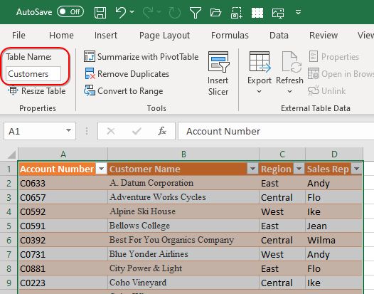
On each of the three worksheets, select the individual data set and press Ctrl+T. Excel will ask you to verify that your data has a header row. Click OK to create the table. By default, these three tables will be called Table1, Table2, and Table3. You can easily change the name of each table before you build the relationships: Select a cell in the table. A Table Design tab appears in the ribbon, and the Table Name can be edited in a box on the left side of the ribbon. For this example, call the three data sets “Data,” “Products,” and “Customers.”

DEFINE RELATIONSHIPS

If you’re using Excel 2016 or newer, you’ll see a Relationships icon in the Data Tools section of the Data tab of the ribbon.

Click the Relationships icon to open the Manage Relationships dialog. On the right side of the Manage Relationships dialog, click New… to create the first relationship.

In the Create Relationship dialog, specify the Data table has a column called ProdID. It’s related to the Products table using the column called Product.

Click New… again and define a second relationship. This one should specify that the Data table has a CustID column that’s related to the Account Number column in the Customers table.

After creating both relationships, they’ll be listed in the Manage Relationships dialog. Click Close to close this dialog.

CREATE THE PIVOT TABLE

This next step is counterintuitive because most people start a pivot table by selecting the data that they want to appear in the pivot table. But for our purposes, you need to insert a blank worksheet in your workbook or simply start from a blank cell on Sheet1 and go to Insert, PivotTable.

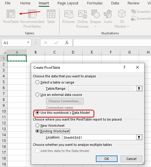
When you start from a blank cell after defining relationships, the Create PivotTable dialog will default to “Use This Workbook’s Data Model.” This sentence always seems cryptic to me. What’s a data model? The answer is that by creating relationships, you unknowingly created a data model that lives in the workbook. The data model contains pointers to the three tables and defines the relationships between those tables.

The first thing you’ll notice in the PivotTable Fields pane is a list of table names instead of a list of field names. Each table has a greater than sign (>) to the left of the table name. Click that icon to reveal the fields available in the table.

SELECT FIELDS FROM ANY TABLE

The power of the data model happens here. You can choose Quantity from the Data table, Region from the Customer table, and Vendor from the Products table. Microsoft will join the data from the three tables much like a query in Access or SQL Server. You don’t have the overhead of thousands of VLOOKUPs.

In the pivot table shown in Figure 2, the vendor names in column A come from the Product table on Sheet2. The Regions shown in row 2 are from the Customers table on Sheet3. The quantities reported in cells B3:E8 are from the invoice register on Sheet1.

STEPS IN EXCEL 2013

The Data Model was brand new in Excel 2013, and there was no obvious way to create a relationship before you built the pivot table. In Excel 2013, you would convert all three sheets to tables. From the table on Sheet1, choose Insert, Pivot Table and choose the box for “Add This Data to the Data Model.” In the PivotTable Fields pane, change from Active to All to reveal all three tables.

As soon as you select fields from more than one table, a yellow warning box appears in the PivotTable Fields pane with a button to Create Relationships. The process feels backwards compared to the easier workflow introduced in Excel 2016, but if you’re still stuck using Excel 2013, it will work.

OTHER DATA MODEL BENEFITS

There have always been two types of pivot tables. A normal pivot table based on data from a single worksheet is a Pivot Cache pivot table. A pivot table created from external data is treated as an OLAP pivot table, and a number of pivot-table features only work with OLAP pivot tables.

When you create a relationship between tables, Excel sees your data as being an external data set. This enables features such as Include Filtered Items in Totals and Distinct Count or the ability to convert the pivot table to Cube Formulas, create subsets of rows or columns, and define new calculations with the DAX formula language.

Joining worksheets in the Data Model brings the relational power of Access or SQL Server to Excel.

About the Authors

February 2020

• Technology & Analytics
• Reporting & Control
• Information Systems
• Financial Recordkeeping
• pivot tables
• advanced Excel tips
• Microsoft Excel
• accounting technology
• how to analyze data in Excel
• Microsoft Office
• Excel Workbook
• IMA Excel 365
• tips in ten
• career development

Publication Highlights

House Passes Corporate Diversity Bill

Explore more.

Copyright Footer Message

Lorem ipsum dolor sit amet

How to Create a Pivot Table in Excel: Step-by-Step (2024)

If you have a huge dataset that’s spread across your entire sheet, and now you want to create a summary out of it – you need a Pivot Table 💪

Pivot Tables make one of the most powerful and resourceful tools of Excel. Using them, you can create a summary out of any kind of data (no matter how voluminous it is).

You can sort your data, calculate sums, totals, and averages and even create summary tables out of it. If you are new to the concept of Pivot Tables, you’d be jaw-dropped by the end of this article.

So you’re ready? Let’s go.

Aa aah! Have you downloaded our free sample workbook for this guide? Get your hands on it right now to practice along with the guide below 🤟

Table of Contents

What is a pivot table?

How to create a pivot table

That’s it – Now what?

Frequently asked questions.

An Excel pivot table is meant to sort and summarize large (very large sets of data).

Once summarized, you can analyze them, make interactive summary reports out of them and even manipulate them 📝

Let’s cut down on the talking and see what a pivot table looks like. Here’s the image of some data in Excel.

The data is about the sales of many products made throughout the year 📆

Yes, it’s super huge and it goes across many columns and rows. But it’s hard to understand the data this way. How about we create a summary of the same?

Wow! That’s what we call a Pivot Table.

It summarizes the sales for each product for each type of customer 💁‍♀️

You can change fields to summarize this data in any way you like. Like summarizing the sales for any particular product, period, type, etc.

Pivot Tables can help you do the following 👇

• Cleanly summarize huge datasets.
• Categorize your data into multiple categories and sub-categories.
• Extract a certain portion of your data (if need be) by selecting the relevant fields only.
• Get any part of your data as a row or as a column (called ‘pivoting’).
• Get totals, and subtotals, or drill down any of them to see their details.

How to create a pivot table in Excel

If the images above made you feel like it would be a science to create a Pivot Table in Excel – that’s just not true.

Pivot Tables are super easy to create. Let me show you how we created the one above 👀

So here’s the data for sales of different products made throughout the year.

Before we go on making a Pivot Table, here are some tips for you to follow to make your Pivot Table better 😎

• Turn your source data into an Excel table before making a Pivot Table out of it. This way, whenever you make any changes to the source data (adding or deleting rows or columns), your Pivot Table will reflect the same.
• Delete any empty rows or columns from the source data.
• Name each column as desired to have the same header as a field title in the Pivot Table.
• Ensure your source data doesn’t have any subtotals or totals.

Let’s concise them into a Pivot Table here.

• Go to the Insert tab > Pivot Tables.

You’ll see the Insert PivotTables dialog box on your screen as follows:

• Create a reference to the cells containing the relevant data.

We will navigate to the sheet ‘Data’ in our workbook and select the cells that contain data.

We have converted our data into an Excel table so Excel automatically recognizes it as Table1. Do not forget to include the headers in the selection.

• Choose the option for New Worksheet or Existing Worksheet.

We will choose New Worksheet to have the Pivot table created on a new sheet.

• Click Okay.

There comes the Pivot Table pane to the right of your sheet 💭

It has two parts. The first part (as above) has all the fields (columns) of your source data listed.

And here’s the second part.

This part includes four boxes where you can specify how each field is to be shown in the Pivot Table. You can choose to have any field organized as a row or as a column, as a filter, or as a value 🎯

• Drag the filed Products from the list of fields to the box for Rows.

Here are the results.

Excel organized all the products as rows.

• Drag the field Amount from the list of fields to the box for Values.

And this is what happens:

Excel adds a column for Values. The column Amount in our source data contained the sales amount of each transaction.

By adding it as values, Excel has summarized the sales of each product and listed them against each of the products 💰

But what if you don’t need the sum of sales of each product, but their count?

• Right-click on any number from the column Sum of Amounts.
• From the context menu, select Summarize Values By.
• Click on any operation that you want to be performed. For example, we want the Count of sales so we are selecting Count 🔢

The results change as follows:

The column Sum of Amounts becomes Count of Amounts . For each product, we now have the Count of sales transactions.

No, it doesn’t stop here.

• Drag the field for Customer Type to the box for columns.

Excel adds columns for each Customer Type . And the sales of each product are now split into customer types 📊

Let’s add another field to see how you can further drill down into details using a Pivot Table.

• Drag and drop the field for Months to the box for Rows.

Excel adds a breakup of months under each product.

So now you can see a summary of sales of each product, for each month and by each customer type. Too convenient and clean ✔

You can make so many more variations to your Pivot Table by pivoting between rows and columns. No matter how vast your data is, Pivot Tables know how to knit it all together.

I am sure you loved the idea of Pivot Tables explained in the Pivot Table tutorial above. Excel Pivot Tables are a blessing for the people who get to deal with huge, messy data now and again.

But that’s just one tool of Excel. And Excel is a whole package of mind-boggling tools, features, and functions. We yet have so much more to explore 🚀

To begin exploring this giant spreadsheet software, I suggest you go with the VLOOKUP, SUMIF, and IF functions of Excel.

Want to learn them already? Enroll in my 30-minute free email course here that will teach you these (and many more) Excel functions in the most fun way.

Other resources

Using pivot tables, you can also create Excel Dashboards. It’s like combining multiple pivot tables in the form of interactive charts and graphs on one page.

Excel dashboards are just amazing – learn how to make them in Excel here.

Also, make sure to check out the 6 best dashboard templates I’ve found on the web!

What is a Pivot Table in Excel used for?

Pivot Tables are used to sort and summarize large datasets in Microsoft Excel. They allow changing pivot table fields so you can readily decide which part of your dataset is to be summarized.

By changing fields, you can create interactive summaries that will bring together massive sets of data in the cleanest manner.

What is the easiest way to add a Pivot Table to your spreadsheet?

To add a Pivot Table to your spreadsheet, go to the sheet (the first cell) where you want the Pivot Table summary inserted.

• Go to the Insert Tab > Pivot Table (Or press the Alt Key > N > V ) to launch the insert Pivot Table dialog box.
• Refer to the cells containing the data.
• Check the option for a ‘New Worksheet’.

• Ablebits blog
• Pivot Table

How to use Pivot Tables in Excel - tutorial for beginners

In this tutorial you will learn what a PivotTable is, find a number of examples showing how to create and use Pivot Tables in all version of Excel 365 through Excel 2007.

If you are working with large data sets in Excel, Pivot Table comes in really handy as a quick way to make an interactive summary from many records. Among other things, it can automatically sort and filter different subsets of data, count totals, calculate average as well as create cross tabulations.

Another benefit of using Pivot Tables is that you can set up and change the structure of your summary table simply by dragging and dropping the source table's columns. This rotation or pivoting gave the feature its name.

What is a Pivot Table in Excel?

An Excel Pivot Table is a tool to explore and summarize large amounts of data, analyze related totals and present summary reports designed to:

• Present large amounts of data in a user-friendly way.
• Summarize data by categories and subcategories.
• Filter, group, sort and conditionally format different subsets of data so that you can focus on the most relevant information.
• Rotate rows to columns or columns to rows (which is called "pivoting") to view different summaries of the source data.
• Subtotal and aggregate numeric data in the spreadsheet.
• Expand or collapse the levels of data and drill down to see the details behind any total.
• Present concise and attractive online of your data or printed reports.

How to make a Pivot Table in Excel

Many people think that creating a Pivot Table is burdensome and time-consuming. But this is not true! Microsoft has been refining the technology for many years, and in the modern versions of Excel, the summary reports are user-friendly are incredibly fast. In fact, you can build your own summary table in just a couple of minutes. And here's how:

1. Organize your source data

Before creating a summary report, organize your data into rows and columns, and then convert your data range in to an Excel Table. To do this, select all of the data, go to the Insert tab and click Table .

Using an Excel Table for the source data gives you a very nice benefit - your data range becomes "dynamic". In this context, a dynamic range means that your table will automatically expand and shrink as you add or remove entries, so won't have to worry that your Pivot Table is missing the latest data.

Useful tips:

• Add unique, meaningful headings to your columns, they will turn into the field names later.
• Make sure your source table contains no blank rows or columns, and no subtotals.
• To make it easier to maintain your table, you can name your source table by switching to the Design tab and typing the name in the Table Name box the upper right corner of your worksheet.

2. Create a Pivot Table

This will open the Create PivotTable window. Make sure the correct table or range of cells is highlighted in the Table/Range field. Then choose the target location for your Excel Pivot Table:

• Selecting New Worksheet will place a table in a new worksheet starting at cell A1.

• In most cases, it makse sense to place a Pivot Table in a separate worksheet , this is especially recommended for beginners.

• It might be useful to create a Pivot Table and Pivot Chart at the same time. To do this, in Excel 2013 and higher, go to the Insert tab > Charts group, click the arrow below the PivotChart button, and then click PivotChart & PivotTable . In Excel 2010 and 2007, click the arrow below PivotTable , and then click PivotChart .

3. Arrange the layout of your Pivot Table report

The area where you work with the fields of your summary report is called PivotTable Field List . It is located in the right-hand part of the worksheet and divided into the header and body sections:

• The Field Section contains the names of the fields that you can add to your table. The filed names correspond to the column names of your source table.
• The Layout Section contains the Report Filter area, Column Labels, Row Labels area, and the Values area. Here you can arrange and re-arrange the fields of your table.

The changes that you make in the PivotTable Field List are immediately reflected to your table.

How to add a field to Pivot Table

By default, Microsoft Excel adds the fields to the Layout section in the following way:

• Non-numeric fields are added to the Row Labels area;
• Numeric fields are added to the Values area;
• Online Analytical Processing (OLAP) date and time hierarchies are added to the Column Labels area.

How to remove a field from a Pivot Table

To delete a certain field, you can either:

• Uncheck the box nest to the field's name in the Field section of the PivotTable pane.
• Right-click on the field in your Pivot Table, and then click " Remove Field_Name ".

How to arrange Pivot Table fields

You can arrange the fields in the Layout section in three ways:

4. Choose summary function for Values (optional)

By default, Microsoft Excel applies the Sum function to numeric value fields placed in the Values area. Conversely, for non-numeric data (such as text, dates, or Boolean values), the Count function is automatically applied.

However, you are free to choose a different summary function according to your preference. For this, right-click on the value field you wish to modify, select Summarize Values By , and then choose the desired function from the options provided.

The functions' names are mostly self-explanatory:

• Sum - calculates the sum of the values.
• Count - counts the number of non-empty values (works as the COUNTA function).
• Average - calculates the average of the values.
• Max - finds the largest value.
• Min - finds the smallest value.
• Product - calculates the product of the values.

5. Show different calculations in value fields (optional)

Excel Pivot Tables provide one more useful feature that enables you to present values in different ways, for example show totals as percentage or rank values from smallest to largest and vice versa. The full list of calculation options is available here .

Tip. The Show Values As feature may prove especially useful if you add the same field more than once and show, for example, total sales and sales as a percent of total at the same time. See an example of such a table.

Working with PivotTable Field List

The Pivot Table pane, which is formally called PivotTable Field List , is the main tool that you use to arrange your summary table exactly the way you want. To make your work with the fields more comfortable, you may want to customize the pane to your liking.

Changing the Field List view

Closing and opening the PivotTable pane

Closing the PivotTableField List is as easy as clicking the Close button (X) in the top right corner of the pane.Making it to show up again is not so obvious :)

Using Recommended PivotTables

As you have just seen, creating a Pivot Table in Excel is easy. However, the modern versions of Excel take even a step further and make it possible to automatically make a report most suited for your source data. All you have to do is 4 mouse clicks:

• Click any cell in your source range of cells or table.
• On the Insert tab, click Recommended PivotTables . Microsoft Excel will immediately display a few layouts, based on your data.
• In the Recommended PivotTables dialog box, click a layout to see its preview.

As you see in the screenshot above, Excel was able to suggest just a couple of basic layouts for my source data, which are far inferior to the Pivot Tables we created manually a moment ago. Of course, this is only my opinion and I am biased, you know : )

How to use Pivot Table in Excel

You can also access options and features that are available for a specific element by right-clicking on it.

How to design and improve Pivot Table

Once you have created a Pivot Table based on your source data, you may want to refine it further to make powerful data analysis.

To improve the table's design, head over to the Design tab where you will find plenty of pre-defined styles. To create your own style, click the More button in the PivotTable Styles gallery, and then click " New PivotTable Style...".

To customize the layout of a certain field, click on that field, then click the Field Settings button on the Analyze tab in Excel 2013 and higher ( Options tab in Excel 2010 and 2007). Alternatively, you can right click the field and choose Field Settings from the context menu.

How to get rid of "Row Labels" and "Column Labels" headings

When you are creating a Pivot Table, Excel applies the Compact layout by default. This layout displays " Row Labels " and " Column Labels " as the table headings. Agree, these aren't very meaningful headings, especially for novices.

How to refresh a Pivot Table in Excel

Although a Pivot Table report is connected to your source data, you might be surprised to know that Excel does not refresh it automatically. You can get any data updates by performing a refresh operation manually, or have it refresh automatically when you open the workbook.

Refresh the Pivot Table data manually

• Click anywhere in your table.

To refresh all Pivot Tables in your workbook, click the Refresh button arrow, and then click Refresh All.

Note. If the format of your Pivot Table gets changed after refreshing, make sure the " Autofit column width on update" and " Preserve cell formatting on update" options are selected. To check this, click the Analyze ( Options ) tab > PivotTable group > Options button. In the PivotTable Options dialog box, switch to the Layout & Format tab and you will find these check boxes there.

Refreshing a Pivot Table automatically when opening the workbook

• On the Analyze / Options tab, in the PivotTable group, click Options > Options .

How to move a Pivot Table to a new location

How to delete an Excel Pivot Table

If you no longer need a certain summary report, you can delete it in a number of ways.

• If your table resides in a separate worksheet , simply delete that sheet.
• If your table is located along with some other data on a sheet, select the entire Pivot Table using the mouse and press the Delete key.
• Click anywhere in the Pivot Table that you want to delete, go to the Analyze tab ( Options tab in Excel 2010 and earlier) > Actions group, click the little arrow below the Select button, choose Entire PivotTable , and then press Delete.

Note. If any PivotTable chart is associated with your table, deleting the Pivot Table will turn it into a standard chart that can no longer be pivoted or updated.

How to prevent pivot table columns from resizing on every change or refresh

By default, Excel pivot tables automatically resize their columns to fit the contents whenever there's a change or refresh. This includes almost every action like adding or removing fields, filtering with drop-down menus, slicers and timelines , or making layout adjustments. While this automatic resizing can be helpful in some situations, it becomes really annoying when the worksheet contains other data outside the pivot table.

Thankfully, there's a simple setting to disable the auto-fit columns feature:

• Right-click any cell inside the pivot table.
• Choose PivotTable Options... from the context menu.
• On the Layout & Format tab, unselect the Autofit column widths on update checkbox.
• Press OK to confirm the change.

Pivot Table examples

The screenshots below demonstrate a few possible Pivot Table layouts for the same source data that might help you to get started on the right path. Feel free to download them get a hands-on experience.

Pivot Table example 1: Two-dimensional table

• Rows: Product, Reseller
• Columns: Months
• Values: Sales

Pivot Table example 2: Three-dimensional table

• Filter: Month
• Rows: Reseller
• Columns: Product

Pivot Table example 3: One field is displayed twice - as total and % of total

• Values: SUM of Sales, % of Sales

Hopefully, this Pivot Table tutorial has been a good starting point for you. If you want to learn advanced features and capabilities of Excel Pivot Tables, check out the links below. And thank you for reading!

Available downloads:

You may also be interested in.

• How to remove Excel table formatting
• How to insert a hyperlink to another worksheet
• Data table in Excel - how to create and use

Table of contents

31 comments

I have many columns. After I create the Pivot Table, I want to apply Show Values As ---> % of Grand Total. But when I select all the columns, and then I apply Show Values As ---> % of Grand Total ... it only applies it to the first column !!! Why? To complete my task, I had to manually do this on each column separately, it took me a long time. How do I apply Show Values As to all columns at once?

Hi! Each column in the Pivot Table needs to be customized individually.

When viewing the data behind a pivot table value as a new worksheet is it possible to select the fields (columns) to be shown as in a power query? In other words, if the original dataset contains 50 columns how can I restrict the new worksheet to show only 5 selected columns of data rather than all 50? This is to avoid having to manually delete 45 columns of unwanted data from the new worksheet.

Hi! If I understand the problem correctly, you can only select the columns you want in PivotTable Field List.

Reviewing the above a few times, it appears this seminar does NOT assist the user as far as INSERTING a row into an existing PivotTable. I created a PivotTable on 01/25/23 and on 2/5/23 needed add a row to the existing table. Did I miss "Insert Row / Columns" section in the above seminar????

Hi! What you can use the pivot table for, is described in detail in the article above. But if you don't need it for your purposes, you don't have to use it. Using the PivotTable Field List, you can add and remove rows from the pivot table.

Spent the entire weekend reviewing your Excel PivotTable seminar(s). Have two questions I can't find answers to. 1) How to add a row to an existing Excel Table (Excel 2007 and 2010 and 2013 and Higher) 2) I have a Excel worksheet with 10 tabs each maintaining detailed schedule. The Summary tab (First tab) contains a Summary Table Hyperlinking total / detail from the other tabs. As I update the low tab, the maintain is updated automatically. Given this fact, why should I create and maintain a Excel PivotTable?? What exactly is the benefit(s) of the PivotTable over the design Hyperlink Master Table?

Basically WHY TAKE TIME TO CREATE A PIVOTTABLE?

In my opinion, the main benefit is that a pivot table allows you to quickly summarize huge amounts of data by categories and subcategories, making it a lot easier to analyze large datasets.

I've looked for a long time for a specific solution to my problem but haven't found one, so here it is:

For those who have been struggling to locate the source of the pivot table in excel when the source is a name, not a cell area.

-> 1) You need to unhide most of the sheets in your file.

2) Go to the drop-down list right above cell A1 in the sheet where your pivot table is located.

3) Click on the name of the source.

4) If it doesn't locate the source right away, continue to unhide sheets. repeat the process listed above.

5) Thank me later.

Pivot table information is very weldon. Clearly we are clarified, So thank you very much your valuable information.

Interested to know more about usage of Pivot Tables in Excel.

Sir in a pivot table can we have present month and cumulative month calculation in one column down by down i.e., A2 has month and A3 cumulative month . Please reply Sir

After delete row from the source data in pivot table, when I refresh in pivot report, I find that source data link is not working, please suggest how I solve this problem.

The below content was very useful for me.

"Another solution is to go to the Analyze (Options) tab, click the Options button, switch to the Display tab and uncheck the "Display Field Captions and Filter Dropdowns" box. However, this will remove all field captions as well as filter dropdowns in your pivot table."

Thankyou very much.

Regards Naresh Prajapati

to expertise in excel

Thank you very much Svetlana Cheusheva and ablebits.com. your posts about excel is very helpful, clean, clear and comprehensive. when I nee to look something about excel I just point my browser to ablebits.com, keep it up. Even Microsoft itself could not give support like yours.

What does it mean by filter, value, column, and row and what do you put in these areas.

I need to put the count of row and sum of person for same data in single pivot chart..... please suggest how can apply this in single pivot for showing two different different count in single pivot. please help me to resolve the same ASAP.

Warm Regards, Yogesh Tandon

Could you help me find a solution for formatting a pivot chart? I did a dash board that contain one chart with primary and secondary axis, and this chart it's attached to a slicer. The problem is: Every time a choose a blank series in the slicer, the chart looses the secondary axies configuration.

Can you Help me? Sorry if it does not sound clear.

To prevent automatic adjustment of the chart's size based on slicer selections, fix the axis bounds (i.e. the starting and ending points of the axes). Please see: How to change the axis scale in Excel chart .

Hi I want to know the short key return pivot table to excel page. If possible please let me know. Thanks.

How to draw pivot tables from 3 different workbooks.Pl. help me.

Great instructions thank you, really clear and easy to understand. Having now got my pivot tables working i would like to use one of the pivot table columns as the source data for a separate drop down menu. Getting the drop down to use the cells as the source is simple but when the pivot table updates and the number of rows changes the drop down does not dynamically update to match so you either end up with blank drop down options or not all options available. Can you help?

I have a list of data having as many 10 rows and two columns. This may be termed as a reference table. Now I have a task by datas used in first table I have to update a very large table containing 25000 and more rows . It took too much time for me to do the task. Please suggest and efficient way to do the same

Perfect exmaple. I have been using this site from quite a long time and i have learned a lot.....

Im trying pivot table but (Range&source) create a problem how to fix this problem please help me

As usual, _great_ instructions. I've been out of the loop a bit with Excel, and they've really added some powerful and cool features to the product.

One minor typo in the instructions - it should be 'Insert' instead of 'Inset' in the line below. To do this, select all of the data, go to the {Inset} tab and click Table.

Anyway, impressive work, thanks very much!!

Thank you, Kupci,

Hi- I am trying to create a pivot for survey responses.... the answers to one of the questions is actual text responses such as "Excellent, Good, ect." Is there an easy way to sort these responses in a pivot? The remaining questions on the survey are numeric responses ranging 1-5, those are working great. It's the text one I am struggling with. Thanks, Deb

Hello, Deb,

To be able to assist you better, we need to see your data. You can send us a small sample table to [email protected] .

Wow. What a wonderful explanation. Thank you very much.

Post a comment

How to Create a Pivot Table Based on Multiple Tables in Excel 2013

Up until recently, if you had data spread across several tables in Microsoft Excel that you wanted to consolidate in a single pivot table, you would have faced a headache-inducing process of manual formatting and data preparation. The most recent version of the software, Excel 2013, fixes this problem by allowing you to create a pivot table from multiple tables automatically -- no manual formatting required. Just follow these steps to get started.

• Learn how to Remove Duplicate Entries and how to add decimal points in Excel
• Here's how to Add a Drop-Down List in Excel
• See how to use Conditional Formatting in Excel to Color-Code Specific Cells

1. Click "Insert"  at the top of the screen.

2. Click the "PivotTable" button  on the Ribbon.

3. Select the first table  you want to add to the pivot table.

4. Check the box labeled "Add this data to the Data Model" and press OK.

5. Click "All"  in the PivotTable Fields window to view all of the tables. Excel automatically detects multiple tables, so you won't need to repeat these steps for each additional table.

6. Check the boxes  of the cells you wish to include in the pivot table.

Stay in the know with Laptop Mag

Get our in-depth reviews, helpful tips, great deals, and the biggest news stories delivered to your inbox.

• 15 PC-Cleaning Tools to Speed Your Computer
• 8 Essential Tips for Your New Windows 8 PC
• 8 Laptop Buying Tips for Students

How to convert PDF to JPG, PNG, or TIFF

How to add Outlook Calendar to Google Calendar

ChromeOS may add 3 cutting-edge features to Chromebook

Most Popular

• 2 Amazon knocks $50 off iPad Pro M4 preorders
• 3 Best MacBook deals in May 2024: Up to $500 off
• 4 Apple Memorial Day sale 2024: MacBook, iPad, Apple Watch, AirPods, more
• 5 Meta Quest’s new Travel Mode makes one overlooked Vision Pro feature even better

Excel Pivot Tables

by contextures.com

Create Two Pivot Tables on Excel Worksheet

In a comment on this blog, someone asked how to create two pivot tables on the same Excel worksheet.

NOTE : See the updated version of this Two Pivot Tables article , from July 2020.

Shown below is a worksheet named Pivot_Reports, with a pivot table on it, based on the data on the Sales_East sheet.

We’ll add another pivot table to the Pivot_Reports sheet, based on data on the Sales_North sheet.

Add the Second Pivot Table

• Select the Sales_North sheet, and select a cell in the data table.
• On the Ribbon, click the Insert tab
• In the Tables group, click PivotTable (click the top half of the PivotTable command).
• In the Create PivotTable dialog box, at the top, leave the default selection of Select a Table or Range, where the Sales_North table shows.
• In the lower section, click Existing Worksheet.
• Click in the Location box, then click on the sheet tab for the Pivot_Reports sheet.
• Click on the cell where the second pivot table should start.
• Click OK to create the new pivot table.
• Add the fields that you’d like in the new pivot table.

The second pivot table is added to the Pivot_Reports worksheet.

Prevent Pivot Table Overlap

When you have two or more pivot tables on the same worksheet, be careful to prevent them from overlapping.

Before you add new fields to the pivot table on the left, you might have to add blank columns between the pivot tables. Or, if one pivot table is above the other, add blank rows between them.

If the pivot tables will change frequently, adding and removing fields, it may be better to keep the pivot tables on separate sheet.

This short video shows pivot table refresh problems, and how to avoid them. For detailed written notes, go to the Pivot Table Errors page on my Contextures site .

Related Articles

Create a Pivot Table In Excel

Create Two Pivot Tables On Excel Worksheet

____________

6 thoughts on “Create Two Pivot Tables on Excel Worksheet”

Can someone advise if it’s possible to be able to insert some data manually in a pivot table that can then be included in the calculations using the calculated field option? I have some data that is not drawn from our finance system that I need to add manually and want to keep it neat with as little manual manipulation as possible.

Hope you’ve gotten an answer by now, but anyway, if you are using Excel 2007, on the Pivot Table Tools, Options ribbon (when your cursor is in the table), in the Tools section of the ribbon, select Formulas and you can create any formula you want to add as a field and put it anywhere in the table you want. Really slick!

Thanks Kathryn, but I’m using 2003; any ideas?

@Paul, you can create a calculated field, but only with data from the pivot table source data, or amounts that you type into the formula, e.g. Bonus= SalesAmt* 0.05

On another sheet, could you use the GetPivotData function to pull results from the pivot table, and combine those values with manual entries?

Is it posible to have two pivot tables in the same worksheet to work with one set of filters?

Good Very usefull data for me. I like this

Leave a Reply Cancel reply

Your email address will not be published. Required fields are marked *

This site uses Akismet to reduce spam. Learn how your comment data is processed .

You are here

Search form, how to update or add new data to an existing pivot table in excel.

This lesson shows you how to refresh existing data , and add new data to an existing Excel pivot table . When you create a new Pivot Table, Excel either uses the source data you selected or automatically selects the data for you. But data changes often, which means you also need to be able to update your pivot tables to reflect the new or changed data.

Scenario: you have a pivot table containing sales data that needs updating with new data

In order to demonstrate how to update the data in your pivot table, let's look at the example we used in our lesson on How to Create A Pivot Table (link opens in a new window), where we summarized several months of sales data by different sales people in our team.

The situation now is that we have been given some additional data and need to incorporate this into our report. Specifically, we've been asked to include sales data for an additional line of products (televisions) for the same time period as the original report.

Here's a sample of the sales data we used (note the number of rows - obviously there is a lot more sales data in our report than is shown here):

And here's the resulting Pivot Table:

Change the Source Data for your Pivot Table

In order to change the source data for your Pivot Table, you can follow these steps:

• The Refresh button will update your pivot table to reflect any changes in your existing data , such as any changes to our sales data due to customer returns. Using the Refresh button won't automatically pick up any new data in your table (unless you're using Excel's Table feature as the source for your pivot table - we'll come to that shortly). Note that you can also choose to refresh your data by right-clicking anywhere in your pivot table and choosing Refresh from the menu.
• The Change Data Source button will allow you specify a new data source for your pivot table. This is the option we want. Note that we're not actually changing to a new data source, we're simply going to update the existing data source to include the new data.

• Manually enter the correct data range for your updated data table. In our case, this would mean changing 693 to 929, since the last row of our table has changed from row 693 to row 929.
• Select the new range from the Data worksheet by selecting all the cells you want to include.

• This uses one of Excel's tricks for quickly selecting large amounts of data (link opens in a new window).
• It keeps the current selection, and extends it by jumping down the spreadsheet to the first blank cell in column A, and stops on the last cell before that.
• Note that this only works if your new data has a value in every row in column A. In our example, we can assume this is the case since the column A holds the date each sale was made.

• Assuming the correct data range has been selected, you can now click OK to update your Pivot Table.
• If you get it wrong, and the wrong data range has been selected, don't panic! Simply try again to select the correct range OR click Cancel and start again OR press CTRL + Z to undo the change.

Some points to remember about updating the data in your pivot tables:

• You don't need to sort your data to when updating the pivot table. In our example, we added the Television data to the end of the existing data, and didn't sort by sales date. The pivot table updated just fine.
• You can choose any data range when updating your pivot table. We added new data to the existing table. We could just as easily have created a new data table with all of our data on another worksheet, and changed our pivot table to point at the new data.
• Note that if you do point your pivot table to a new table, your pivot table design may change if the new data table doesn't have the same columns as your original data table. This is where CTRL+Z comes in handy, to undo the change.
• If you're using Excel's Table feature, most of this lesson isn't necessary, since Excel uses the table as the data source, and automatically reflects any changes to the table in the pivot table. However, you will still need to Refresh your pivot table to include the new or changed data in the pivot table.
• Finally, you may have noticed the option to Use an External Data Source. This allows you to use an external database. This is reasonably complicated, and outside the scope of this lesson. Suffice to say that this method generally ensures that your pivot table contains the latest data from your database but, once again, you still need to use the Refresh button to update the pivot table.

If you have any comments on this lesson, or questions about how to update the data in your pivot tables, please feel free to post them in the comments section below.

Want to learn more? Try these lessons:

Our comment policy..

We welcome your comments and questions about this lesson. We don't welcome spam. Our readers get a lot of value out of the comments and answers on our lessons and spam hurts that experience. Our spam filter is pretty good at stopping bots from posting spam, and our admins are quick to delete spam that does get through. We know that bots don't read messages like this, but there are people out there who manually post spam. I repeat - we delete all spam, and if we see repeated posts from a given IP address, we'll block the IP address. So don't waste your time, or ours. One other point to note - if you post a link in your comment, it will automatically be deleted.

Add a comment to this lesson

Comments on this lesson

Additional data.

Is it possible to download the file for the additional data that you are adding to the pivot table in this lesson?

Pivot Table didn't show all data rows after adding new data

Thanks for this topic. I am able to change Data Source to include new data. However, my pivot table didn't show all data rows (some data at the end are hidden) because the pivot table rows keep the same as before. How or what can I do to see all data rows? Thanks, Huilan

Missing pictures of pivot tables

from where you talk about 928 lines all the pivot table pictures are missing - its showing a blue square and your comments only.

Images are back again

Thanks for your post - sorry - the images have been restored now. It may take up to an hour for cached copies of the page to be updated.

Adding new data to PIVOT TABLE

Hi, I was wondering if you can advice me. I added a new row with data (in the middle of the data), and when I refresh the new data is shown in the pivot table as the last row. Is there any way to force the pivot to keep the position in where I inserted the new data?

Is there a way to add a "hit ratio" column, that would divide one column by another to create a hit ratio percentage??

old pivot should get update automatically with new column and da

When we create pivot table after that if we change data source with completely new columns and data, i want only pivot table to update without manually putting columns in pivot table it should refresh column headers and data.

Hi Guys, When i added a new column to my data sheet, some of my existing results (one column) has changed, how can this be fixed or how does this happen?

Any help with this is greatly appreciated!

I want to add a new sales person to my pivot table

How do I do this?

Add comment

• No HTML tags allowed.
• Web page addresses and e-mail addresses turn into links automatically.
• Lines and paragraphs break automatically.

• Skip to primary navigation
• Skip to main content
• Skip to primary sidebar

Technology Simplified.

How to Create Two Pivot Tables in Single Worksheet

By: Waseem Patwegar | Filed Under: Office

Sometimes, you may want to create two Pivot tables in single Excel worksheet to report data in two different ways. You will find below the steps to create Two Pivot Tables in Single Worksheet.

Create Two Pivot Tables in Single Worksheet

As mentioned above, the common reason for creating Two Pivot Tables in Single Worksheets is to analyze and report data in two different ways.

For example, consider the following Sales Data as recorded at 2 different store locations (Store#1 and Store#2).

For above Sales Data, you can Create Two Pivot Table in same Worksheet, reporting or analyzing Sales Data in two different ways.

For example, the First Pivot Table can be configured to report ‘Sales Data by Gadget Type’ and the second Pivot Table to report ‘Sales Data by Store’.

1. Create First Pivot Table

Follow the steps below to create the First Pivot Table to show Sales Data by Products.

1. Select any Cell in the Source Data > click on Insert > Tables and select Recommended PivotTables option.

2. On Recommended PivotTables screen, choose the PivotTable Layout that you want to use and click on OK .

3. Once you click on OK , Excel will insert the first Pivot Table in a new worksheet.

4. Once Pivot Table is inserted, click on any Cell within the Pivot Table and this will bring up the ‘PivotTable Fields’ List.

Modify the first Pivot Table as required by adding and dragging the Field Items between Columns, Rows and Values areas.

2. Create Second Pivot Table in Same Worksheet

Now, you can create a second Pivot Table in the same Worksheet by following the steps below.

1. Click on any empty cell in the same Worksheet – Make sure the Cell is away from the first pivot table that you just created.

2. Next, click on the Insert tab and click on PivotTable  option.

3. On the next screen, select Pivot Table Range , select Existing Worksheet option and click on the OK button to insert a blank Pivot Table in the same Worksheet.

4. Once blank Pivot Table is inserted, build the second Pivot Table as required by selecting items and dragging them between Columns, Rows and Values areas in PivotTable Fields list.

This way, you will end up with two Pivot tables on the same worksheet, reporting sales data in two different ways.

Whenever new sales are added, you can just refresh the two Pivot Tables and this will update the data in both Pivot Tables.

Similarly, you can add as many pivot tables in the same worksheet as you want and report data in different ways.

How to Fix Pivot Table Report Overlap Warning

When you insert two or more Pivot Tables in the same Worksheet, you may come across Pivot Table Report overlap warning, whenever you try to make changes in the Pivot Tables.

If this happens, click on OK to close the warning message and simply space out the two Pivot Tables.

You can space out Pivot Tables by inserting few blank rows (if Pivot Tables are one above another) and by inserting some blank columns (if Pivot Tables are side by side).

If you are going to change Pivot Tables frequently (adding and removing fields), it is better to keep the Pivot Tables on separate worksheets.

• How to Create Pivot Table From Multiple Worksheets
• How to Add or Remove Subtotals in Pivot Table
• Replace Blank Cells with Zeros in Excel Pivot Table

Microsoft Excel Guides

Google sheet guides, productivity resources.

Table of Contents

How to add multiple pivot tables to one sheet in Microsoft Excel

Adding multiple pivot tables to one sheet in Excel can be a useful way to summarize and analyze large amounts of data. With multiple pivot tables on the same sheet, you can easily compare and contrast different aspects of your data and identify trends and patterns that may not be immediately apparent from individual tables.

In this tutorial, we will learn how to add multiple pivot tables to one sheet in Microsoft Excel. Adding multiple pivot tables to one sheet in Excel can be done by creating the first pivot table, clicking on a cell where you want to place the second pivot table, and repeating the process for each additional table. 

Here we have two distinct data sets. We will create a pivot table for each data set on one sheet.

Method 1: Adding Multiple Pivot Tables From Different Data Sets

Step 1 – select the range of cells.

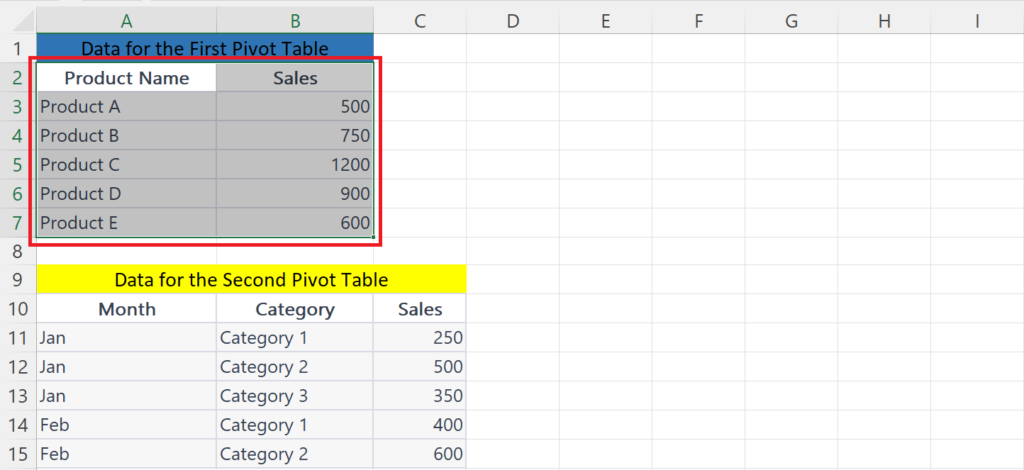
• Select the range of cells containing the source data for the first pivot table.

Step 2 – Go to the Insert Tab

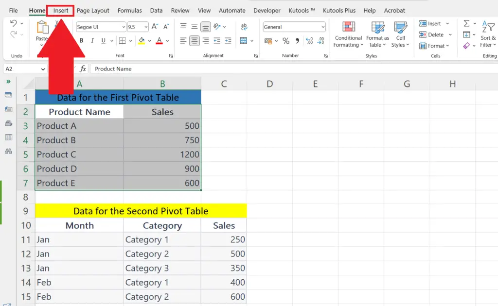
• Go to the Insert tab in the menu bar.

Step 3 – Click on the PivotTable Button

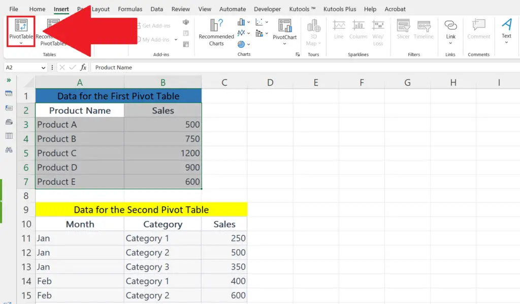
• Click on the PivotTable button on the right end of the ribbon.
• The “PivotTable from table or range” dialog box will appear.

Step 4 – Select the Existing worksheet Option and Enter the Location

• Select the Existing worksheet option.
• Enter the location where you want to place the pivot table.

Step 5 – Click on OK

• Click on OK in the dialog box.
• The first pivot table will be created.

Step 6 – Select the Range of Cells

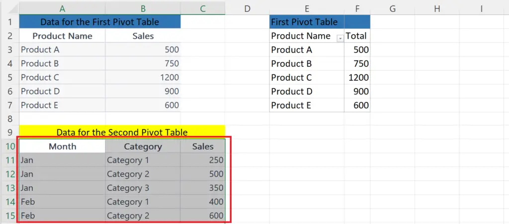
• Select the range of cells containing the source data for the second pivot table.

Step 7 – Go to the Insert Tab

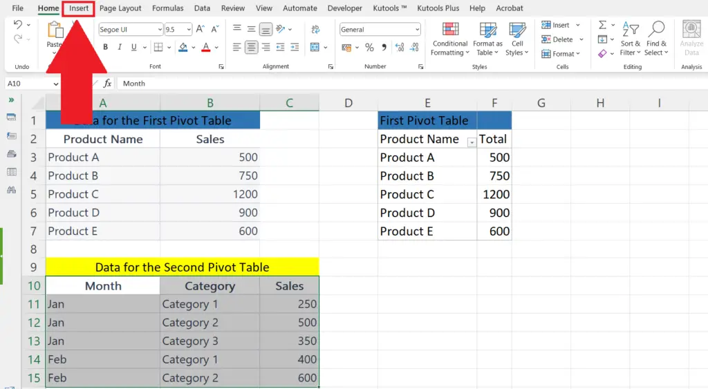
Step 8 – Click on the PivotTable Button

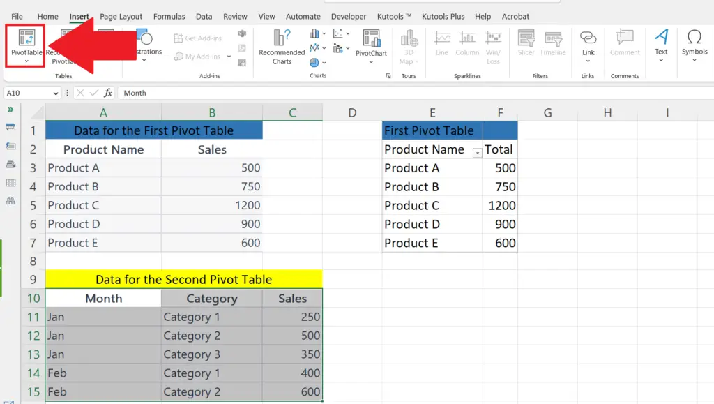
Step 9 – Select the Existing worksheet Option and Enter the Location

Step 10 – click on ok.

• The second pivot table will be created.

Method 2: Adding Multiple Pivot Tables From the Same Data Set for Different Fields

For this method, we will use a data set that represents Sales of products of two categories i.e. Electronics and Fashion done by three salespersons i.e. John, Sarah, and Mary.

We will add two pivot tables i.e. one representing the total sales by each salesperson and the other, representing the total sales of each product.

Step 1 – Select the Data Range

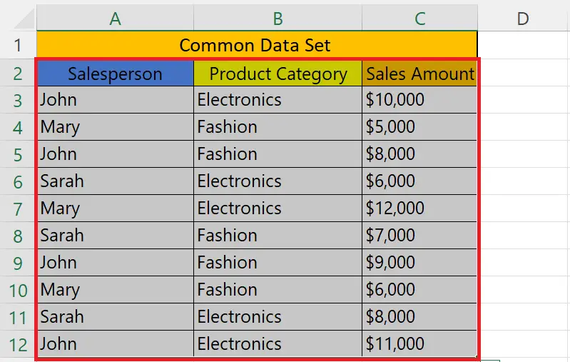
• Select the range of cells containing the data set from which we want to make multiple pivot tables.

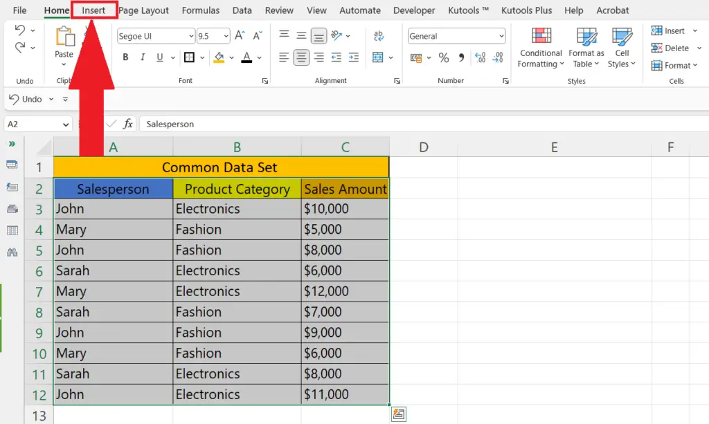
Step 3 – Click on the Pivot Table Button

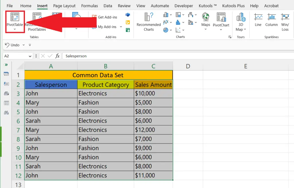
• Click on the Pivot table button at the left end of the ribbon.

Step 4 – Insert the First Pivot Table

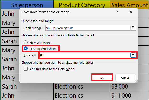
• A dialog box will appear.
• Select the “Existing Worksheet” option and enter the location i.e. E1.
• Click on OK.

Step 5 – Add the Fields for the First Pivot Table

• Add the field for the first pivot table i.e. Sales Person and Sales amount.
• For this, just check the boxes with each option.
• The First pivot table will be added, representing the total sales of each person.

Step 6 – Again Select the Data Range

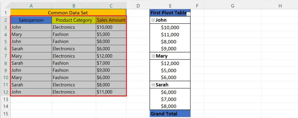
• Select the range of cells containing the data set from which we want to make multiple pivot tables for the second pivot table.

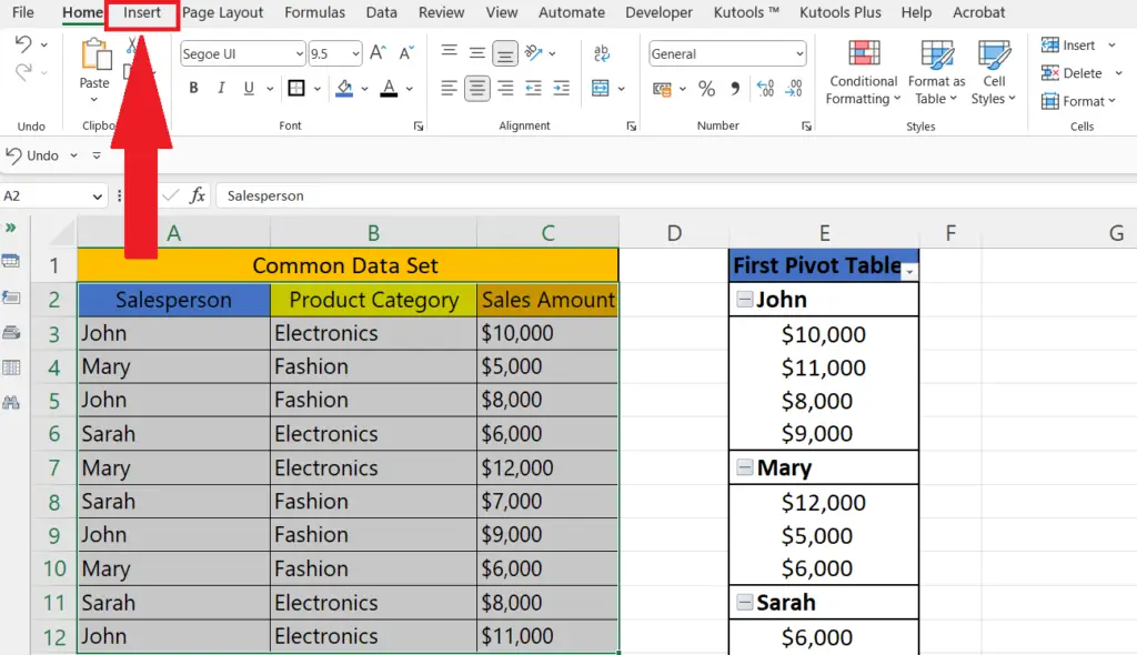
Step 8 – Click on the Pivot Table Button

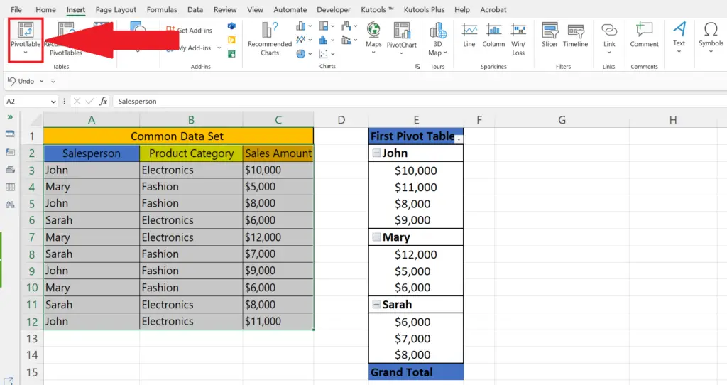
Step 9 – Insert the Second Pivot Table

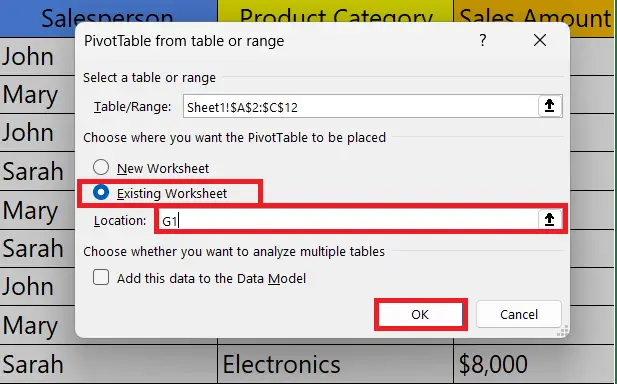
• Select the “Existing Worksheet” option and enter the location i.e. G1.

Step 10 – Add the Fields for the Second Pivot Table

• Add the field for the second pivot table i.e. Product Category and Sales amount.
• The Second pivot table will be added, representing the total sales of each product category.

Related Posts

How to count a range of numbers in excel.

How to transfer data from Microsoft Excel to Microsoft Word

How to scrape data from a website into excel.

• PRO Courses Guides New Tech Help Pro Expert Videos About wikiHow Pro Upgrade Sign In
• EDIT Edit this Article
• EXPLORE Tech Help Pro About Us Random Article Quizzes Request a New Article Community Dashboard This Or That Game Popular Categories Arts and Entertainment Artwork Books Movies Computers and Electronics Computers Phone Skills Technology Hacks Health Men's Health Mental Health Women's Health Relationships Dating Love Relationship Issues Hobbies and Crafts Crafts Drawing Games Education & Communication Communication Skills Personal Development Studying Personal Care and Style Fashion Hair Care Personal Hygiene Youth Personal Care School Stuff Dating All Categories Arts and Entertainment Finance and Business Home and Garden Relationship Quizzes Cars & Other Vehicles Food and Entertaining Personal Care and Style Sports and Fitness Computers and Electronics Health Pets and Animals Travel Education & Communication Hobbies and Crafts Philosophy and Religion Work World Family Life Holidays and Traditions Relationships Youth
• Browse Articles
• Learn Something New
• Quizzes Hot
• This Or That Game
• Train Your Brain
• Explore More
• Support wikiHow
• About wikiHow
• Log in / Sign up
• Computers and Electronics
• Spreadsheets
• Microsoft Excel

How to Add a Column or Calculated Field in an Excel Pivot Table

Quick step-by-step guide to creating a new pivot table column

Last Updated: March 25, 2024 Fact Checked

Changing a Field to Column

Adding a calculated field.

This article was co-authored by wikiHow staff writer, Kyle Smith . Kyle Smith is a wikiHow Technology Writer, learning and sharing information about the latest technology. He has presented his research at multiple engineering conferences and is the writer and editor of hundreds of online electronics repair guides. Kyle received a BS in Industrial Engineering from Cal Poly, San Luis Obispo. This article has been fact-checked, ensuring the accuracy of any cited facts and confirming the authority of its sources. This article has been viewed 671,504 times. Learn more...

This wikiHow teaches you how to insert a new column into a pivot table in Microsoft Excel with the pivot table tools. You can easily change an existing row, field, or value to a column, or create a new calculated field column with a custom formula.

Things You Should Know

• Show the Field List by going to PivotTable Analyze > Field List .
• Drag field items to the Columns area in the Field List to create new columns.
• Go to PivotTable Analyze > Fields, Items, & Sets > Calculated Field to make a custom field.

• If you haven't made your pivot table yet, open a new Excel document and create a pivot table before continuing.

• On some versions, this tab may just be named Analyze , and on others, you can find it as Options under the "Pivot Table Tools" heading.

• Typically, non-numeric fields are added as rows, and numeric fields are added as values.
• You can uncheck the checkbox here anytime to remove the field from your pivot table.

• For example, if you have a column of years called “Years” in your source data, you can add the “Years” field to the Columns area to create columns for each year, showing values for each individual year.
• You can drag the field item name from the list of fields or from another area (Filters, Rows, Values).
• Now you’re ready to analyze the data and make a few charts using the pivot table.

• If you haven't yet made the pivot table, open a new Excel document and create a pivot table before continuing.

• On different versions, this tab may be named Analyze , or Options under the "Pivot Table Tools" heading.

• Make sure you type the formula on the right side of the "=" sign.
• Select the field you want to add in the Fields section.
• Click Insert Field to add it to your formula.
• For example, if you have the fields “revenue” and “costs”, you could subtract them to get a “profit” calculated field.

• Alternatively, click Add to create the calculated field without closing the “Insert Calculated Field” window. This allows you to add additional calculated fields.
• You can reorder the columns by dragging the field items in the pivot table “Column” area.

Expert Q&A

• Make sure to backup your original Excel document before modifying the pivot table. Thanks Helpful 0 Not Helpful 0
• For more helpful Excel guides, check out how to use Vlookup and how to use Solver . Thanks Helpful 0 Not Helpful 0

• Always remember to save your work when you're done. Thanks Helpful 0 Not Helpful 0

You Might Also Like

• ↑ https://support.microsoft.com/en-us/office/create-a-pivottable-to-analyze-worksheet-data-a9a84538-bfe9-40a9-a8e9-f99134456576

About This Article

1. Click on the PivotTable . 2. Click the checkbox of the field you want to add. 3. Right-click on the added field. 4. Select Move to... Column Labels or Values. Did this summary help you? Yes No

• Send fan mail to authors

Is this article up to date?

Featured Articles

Trending Articles

Watch Articles

• Terms of Use
• Privacy Policy
• Do Not Sell or Share My Info
• Not Selling Info

Keep up with tech in just 5 minutes a week!

Guide To How To Add Pivot Table To Existing Sheet

Introduction.

When it comes to data analysis, pivot tables are a valuable tool for organizing and summarizing data in spreadsheets. They allow users to quickly and easily analyze large amounts of data and gain valuable insights. In this blog post, we will discuss the importance of pivot tables in data analysis and provide a brief overview of the steps to add a pivot table to an existing sheet .

Key Takeaways

• Pivot tables are a valuable tool for organizing and summarizing data in spreadsheets
• They allow for quick and easy analysis of large amounts of data
• Adding a pivot table to an existing sheet involves selecting the data range, inserting the pivot table, designing the layout, and refreshing the table as needed
• Pivot tables play a crucial role in effective data analysis in Excel
• Practicing using pivot tables can lead to gaining valuable insights from data

Step 1: Open the existing Excel sheet

Before you can add a pivot table to an existing Excel sheet, you need to open the sheet in Microsoft Excel. Here's how to do it:

To begin, locate the existing Excel sheet on your computer. You may have the file saved in a specific folder or on your desktop. Once you have found the file, double-click on it to open it in Microsoft Excel.

After you have located the file, it's time to open it in Microsoft Excel. If Excel is your default program for opening spreadsheets, you can simply double-click on the file to open it. If not, you can right-click on the file, select "Open with," and choose Microsoft Excel from the list of programs.

Step 2: Select the data range for the pivot table

Once you have identified the data that you want to include in the pivot table, the next step is to select the data range.

A. Highlight the data range that you want to include in the pivot table

Go to the worksheet that contains the data you want to use for the pivot table. Click and drag to highlight the entire range of data that you want to include. This will ensure that the pivot table will be based on the correct data.

B. Ensure there are no blank rows in the selected data range

It is important to ensure that there are no blank rows within the selected data range. Blank rows can cause issues with the pivot table and may result in inaccurate or incomplete data analysis. If there are any blank rows, either remove them or adjust the data range selection to exclude them.

Step 3: Insert a pivot table

After preparing the data and selecting the range, the next step is to insert a pivot table.

Go to the top of the Excel window and click on the "Insert" tab to access the pivot table option.

After clicking on the "Insert" tab, a dropdown menu will appear. From the dropdown menu, select "PivotTable" to begin creating the pivot table.

Once "PivotTable" is selected, a dialog box will appear prompting you to choose the location for the pivot table. You can select whether you want to place the pivot table in a new worksheet or an existing worksheet. Choose the location that best fits your needs.

Step 4: Design the pivot table

Once you have added the necessary fields to the pivot table, it’s time to design the layout and format of the table to meet your specific requirements.

After adding the fields to the pivot table, you can easily rearrange them by dragging and dropping them into the appropriate sections of the pivot table field list. The "Rows" area will display the unique values of the selected field, while the "Values" area will calculate the summary data based on the selected field.

Once the fields are in place, you can customize the layout and format of the pivot table to make it more visually appealing and easier to analyze. This can include adjusting the column widths, applying different styles and themes, and adding subtotals or grand totals as needed.

It is common for blank rows to appear in the pivot table results, especially if there is missing data in the original dataset. To clean up the pivot table, simply filter out the blank rows by unchecking the "blank" option in the filter dropdown menu for the specific field.

Step 5: Refresh the pivot table if the source data changes

After you have successfully created your pivot table, it's important to know how to refresh it if the source data changes. This ensures that your pivot table always reflects the latest information.

To refresh your pivot table, start by right-clicking anywhere within the pivot table.

Once you right-click, a dropdown menu will appear. From this menu, select the "Refresh" option to update the pivot table with the most current data from the source.

Adding a pivot table to an existing sheet is a powerful tool for data analysis in Excel. Pivot tables allow you to quickly summarize and analyze large amounts of data, providing valuable insights for decision-making.

• Recap the steps: First, select any cell in the data range and go to the 'Insert' tab. Then, click on 'PivotTable' and choose the data range. Next, select where you want the pivot table to be placed and drag and drop the fields to organize your data.
• Encourage practice: To become proficient in using pivot tables, practice is vital. Try using different data sets and experimenting with various pivot table options to gain a deeper understanding of their capabilities.

By mastering pivot tables, you can streamline your data analysis process and make more informed decisions based on your findings. Happy analyzing!

Immediate Download

MAC & PC Compatible

Free Email Support

Related aticles

The Benefits of Excel Dashboards for Data Analysts

Unlock the Power of Real-Time Data Visualization with Excel Dashboards

Unlocking the Potential of Excel's Data Dashboard

Unleashing the Benefits of a Dashboard with Maximum Impact in Excel

Exploring Data Easily and Securely: Essential Features for Excel Dashboards

Unlock the Benefits of Real-Time Dashboard Updates in Excel

Unleashing the Power of Excel Dashboards

Understanding the Benefits and Challenges of Excel Dashboard Design and Development

Leverage Your Data with Excel Dashboards

Crafting the Perfect Dashboard for Excel

An Introduction to Excel Dashboards

How to Create an Effective Excel Dashboard

• Choosing a selection results in a full page refresh.

Excel 2024: Make Pivot Tables Expandable Using Ctrl+T

May 15, 2024 - by Bill Jelen

If you choose all of columns A:J and you later want to add more records below the data, it takes only a simple Refresh to add the new data instead of having to find the Change Data Source icon. In the past, this made sense. But today, Change Data Source is right next to the Refresh button and not hard to find. Plus, there is a workaround in the Ctrl+T table.

When you choose your data set and select Format as Table by using Ctrl+T , the pivot table source will grow as the table grows. You can even do this retroactively, after the pivot table exists.

This figure below shows a data set and a pivot table. The pivot table source is A1:C16.

Say that you want to be able to easily add new data below the pivot table, as shown below. Select one cell in the data and press Ctrl+T . Make sure that My Table Has Headers is checked in the Create Table dialog and click OK.

Some nice formatting is applied to the data set. But the formatting is not the important part.

You have some new records to add to the table. Copy the records.

Go to the blank row below the table and paste. The new records pick up the formatting from the table. The angle-bracket-shaped End-of-Table marker moves to C19. But notice that the pivot table has not updated yet.

Click the Refresh button in the Pivot Table Tools Analyze tab. Excel adds the new rows to your pivot table.

Bonus Tip: Use Ctrl+T with VLOOKUP and Charts

In this figure, the VLOOKUP table is in E5:F9. Item A106 is missing from the table, and the VLOOKUP is returning #N/A . Conventional wisdom says to add A106 to the middle of your VLOOKUP table so you don't have to rewrite the formula.

Instead, use Ctrl+T to format the lookup table. Note that the formula is still pointing to E5:F9; nothing changes in the formula.

But when you type a new row below the table, it becomes part of the table, and the VLOOKUP formula automatically updates to reflect the new range.

The same thing happens with charts. The chart on the left is based on A1:B5, which is not a table. Format A1:B5 as a table by pressing Ctrl+T . Add a new row. The row is automatically added to the chart, as shown on the right.

It is fairly cool that you can use Ctrl+T after setting up the pivot table, VLOOKUP , or chart, and Excel still makes the range expand.

When I asked readers to vote for their favorite tips, tables were popular. Thanks to Peter Albert, Snorre Eikeland, Nancy Federice, Colin Michael, James E. Moede, Keyur Patel, and Paul Peton for suggesting this feature. Four readers suggested using OFFSET to create expanding ranges for dynamic charts: Charley Baak, Don Knowles, Francis Logan, and Cecelia Rieb. Tables now do the same thing in most cases.

This article is an excerpt from MrExcel 2024 Igniting Excel

Title photo by Andrei Zolotarev on Unsplash

• Create a PivotTable Video
• Create a PivotTable manually Video
• Sort, filter, and calculate Video
• Use slicers, timelines and PivotCharts Video

Create a PivotTable manually

Create a manual PivotTable if you prefer to design the PivotTable yourself. Here's how.

Create a PivotTable to analyze external data

Create a PivotTable to analyze data in multiple tables

Show different calculations in PivotTable value fields

Create a PivotChart

Available chart types

This table contains data about book sales.

It has a column for the Genre of the books, the Date they were sold, the Sales Amount, and the Store where they were sold.

Before you create a PivotTable, the data you are going to use (referred to as Source Data) should be arranged correctly.

All the columns should have headings. The headings are used to name the fields in the PivotTable.

Each column contains the same type of data, for example, text in one column and currency in another, and there should be no blank rows or columns.

For this PivotTable, we’ll use source data that is in a table.

It doesn’t have to be in a table, a range of cells can be used as well.

For information about using external data, see the article Create a PivotTable to analyze external data .

For information about using multiple database tables, see Create a PivotTable to analyze data in multiple tables .

There’s a link to both articles in the course summary at the end of the course.

Click any cell in the data. Click INSERT and PivotTable . All of the source data is automatically selected. In this example, the entire SourceData table.

We recommend using a table because, if the table grows, the PivotTable will automatically include the new data when you refresh the PivotTable.

For information about creating a table, see the link Create or delete an Excel table in a worksheet in the course summary.

By default, the PivotTable will be created on a New Worksheet .

If you want, you can create it on an existing worksheet instead, by clicking Existing Worksheet and providing the Location . Click OK . In our example, a new worksheet with an empty PivotTable is created.

In the PivotTable Fields List , at the top, are the fields we’ll use to create the PivotTable.

They are the same as the column headings in the source data.

At the bottom are the four areas of a PivotTable; the fields can be added to: ROWS , COLUMNS , VALUES , and FILTERS .

I check the Genre field and it’s added to the PivotTable as rows of text labels.

By default, text fields are added as rows and numbers as values.

Check the Sales Amount field and it’s added as a column of values that are added using the SUM function.

Right-click a cell in the Sum of Sales Amount column, click Number Format , and click Currency .

I don’t want any digits after the decimal place, so I set the Decimal places to 0, click OK , and we can see the total sales for the different genres of books.

I click and drag the Store field to COLUMNS , and we can see the sales of genres for each store along with grand totals.

An important factor we don’t have in the PivotTable yet are dates. How do sales differ over time?

I check the Date field and it’s added to the ROWS area. But this many rows of dates makes the PivotTable hard to use.

Let’s group the list of dates. Right-click any date, and click Group .

I'll use the default, Months , but you can select one or more options, such as Quarters and Years . Click OK .

The dates are grouped under the genres by month, much easier to work with. And we can see the sales of the genres over time for each store.

When you click any cell in a PivotTable, the PivotTable Fields List and the PIVOTTABLE TOOLS tab appear.

When you click outside of the table, they go away.

Under PIVOTTABLE TOOLS , click the DESIGN tab to change how the PivotTable looks.

For example, click Report Layout , click Show in Outline Form , and now Genre and Date are in separate columns.

Check Banded Rows to make it easier to read across the rows of the PivotTable.

Click the down-arrow next to PivotTable Styles ; there are many options.

When you mouse over them, you get a preview of what the PivotTable will look like.

Click the style you want to change the look of the PivotTable.

We’ll cover the ANALYZE tab in subsequent videos.

Up next: Sort, filter, summarize, and calculate your PivotTable data .

Need more help?

Want more options.

Explore subscription benefits, browse training courses, learn how to secure your device, and more.

Microsoft 365 subscription benefits

Microsoft 365 training

Microsoft security

Accessibility center

Communities help you ask and answer questions, give feedback, and hear from experts with rich knowledge.

Ask the Microsoft Community

Microsoft Tech Community

Windows Insiders

Microsoft 365 Insiders

Was this information helpful?

Thank you for your feedback.

Contribute to the Microsoft 365 and Office forum! Click  here  to learn more  💡

April 9, 2024

Contribute to the Microsoft 365 and Office forum!

Click  here  to learn more  💡

Excel Forum Top Contributors: HansV MVP  -  Ashish Mathur  -  Andreas Killer  -  Jim_ Gordon  -  Riny_van_Eekelen   ✅

May 10, 2024

Excel Forum Top Contributors:

HansV MVP  -  Ashish Mathur  -  Andreas Killer  -  Jim_ Gordon  -  Riny_van_Eekelen   ✅

• Search the community and support articles
• Microsoft 365 and Office
• Search Community member

Ask a new question

In a pivot table why does it open up a new tab as 'detail' and not 'sheet' when I double click a summary value

My Pivot table has changed how it gives the detail behind the summary value. Previously by double clicking on the value it would create a new tab with the information making up the summary value, naming it 'sheet2'. I have run the same Pivot today, but when double click on the value, it creates a new tab as 'detail1' and adds two lines at the top of the sheet, with the first line starting with ' Detail for Count____'.

I have got colleagues to run the same Pivot and theirs works fine by creating the tab as 'sheet1', suggesting that the format on my version of Excel has changed. Does anyone know how I can change it back.

• Subscribe to RSS feed

Report abuse

Reported content has been submitted​

Replies (3) 

• Volunteer Moderator

Which version, build (and release channel) are you on?

Was this reply helpful? Yes No

Sorry this didn't help.

Great! Thanks for your feedback.

How satisfied are you with this reply?

Thanks for your feedback, it helps us improve the site.

Thanks for your feedback.

Microsoft® Excel® for Microsoft 365 MSO (Version 2404 Build 16.0.17531.20140) 64-bit

That appears to be the May 7 release for the Current Channel, which is the latest, so I suspect it's a feature update. Presumably your co-workers are not quite as up to date as you are.

Question Info

• For business
• Norsk Bokmål
• Ελληνικά
• Русский
• עברית
• العربية
• ไทย
• 한국어
• 中文(简体)
• 中文(繁體)
• 日本語