Module 6: Algebraic Operations on Functions
Compressions and stretches, learning outcomes.
- Graph Functions Using Compressions and Stretches.
Adding a constant to the inputs or outputs of a function changed the position of a graph with respect to the axes, but it did not affect the shape of a graph. We now explore the effects of multiplying the inputs or outputs by some quantity.
We can transform the inside (input values) of a function or we can transform the outside (output values) of a function. Each change has a specific effect that can be seen graphically.

Vertical Stretches and Compressions
When we multiply a function by a positive constant, we get a function whose graph is stretched or compressed vertically in relation to the graph of the original function. If the constant is greater than 1, we get a vertical stretch ; if the constant is between 0 and 1, we get a vertical compression . The graph below shows a function multiplied by constant factors 2 and 0.5 and the resulting vertical stretch and compression.

Vertical stretch and compression
A General Note: Vertical Stretches and Compressions
Given a function [latex]f\left(x\right)[/latex], a new function [latex]g\left(x\right)=af\left(x\right)[/latex], where [latex]a[/latex] is a constant, is a vertical stretch or vertical compression of the function [latex]f\left(x\right)[/latex].
- If [latex]a>1[/latex], then the graph will be stretched.
- If [latex]0 < a < 1[/latex], then the graph will be compressed.
- If [latex]a<0[/latex], then there will be combination of a vertical stretch or compression with a vertical reflection.
How To: Given a function, graph its vertical stretch.
- Identify the value of [latex]a[/latex].
- Multiply all range values by [latex]a[/latex].
- If [latex]a>1[/latex], the graph is stretched by a factor of [latex]a[/latex]. If [latex]{ 0 }<{ a }<{ 1 }[/latex], the graph is compressed by a factor of [latex]a[/latex]. If [latex]a<0[/latex], the graph is either stretched or compressed and also reflected about the [latex]x[/latex]-axis.
Example: Graphing a Vertical Stretch
A function [latex]P\left(t\right)[/latex] models the number of fruit flies in a population over time, and is graphed below.
A scientist is comparing this population to another population, [latex]Q[/latex], whose growth follows the same pattern, but is twice as large. Sketch a graph of this population.

Because the population is always twice as large, the new population’s output values are always twice the original function’s output values.
If we choose four reference points, (0, 1), (3, 3), (6, 2) and (7, 0) we will multiply all of the outputs by 2.
The following shows where the new points for the new graph will be located.
[latex]\begin{cases}\left(0,\text{ }1\right)\to \left(0,\text{ }2\right)\hfill \\ \left(3,\text{ }3\right)\to \left(3,\text{ }6\right)\hfill \\ \left(6,\text{ }2\right)\to \left(6,\text{ }4\right)\hfill \\ \left(7,\text{ }0\right)\to \left(7,\text{ }0\right)\hfill \end{cases}[/latex]

Symbolically, the relationship is written as
[latex]Q\left(t\right)=2P\left(t\right)[/latex]
This means that for any input [latex]t[/latex], the value of the function [latex]Q[/latex] is twice the value of the function [latex]P[/latex]. Notice that the effect on the graph is a vertical stretching of the graph, where every point doubles its distance from the horizontal axis. The input values, [latex]t[/latex], stay the same while the output values are twice as large as before.
How To: Given a tabular function and assuming that the transformation is a vertical stretch or compression, create a table for a vertical compression.
- Determine the value of [latex]a[/latex].
- Multiply all of the output values by [latex]a[/latex].
Example: Finding a Vertical Compression of a Tabular Function
A function [latex]f[/latex] is given in the table below. Create a table for the function [latex]g\left(x\right)=\frac{1}{2}f\left(x\right)[/latex].
The formula [latex]g\left(x\right)=\frac{1}{2}f\left(x\right)[/latex] tells us that the output values of [latex]g[/latex] are half of the output values of [latex]f[/latex] with the same inputs. For example, we know that [latex]f\left(4\right)=3[/latex]. Then
[latex]g\left(4\right)=\frac{1}{2}\cdot{f}(4) =\frac{1}{2}\cdot\left(3\right)=\frac{3}{2}[/latex]
We do the same for the other values to produce this table.
Analysis of the Solution
The result is that the function [latex]g\left(x\right)[/latex] has been compressed vertically by [latex]\frac{1}{2}[/latex]. Each output value is divided in half, so the graph is half the original height.
A function [latex]f[/latex] is given below. Create a table for the function [latex]g\left(x\right)=\frac{3}{4}f\left(x\right)[/latex].
Example: Recognizing a Vertical Stretch

The graph is a transformation of the toolkit function [latex]f\left(x\right)={x}^{3}[/latex]. Relate this new function [latex]g\left(x\right)[/latex] to [latex]f\left(x\right)[/latex], and then find a formula for [latex]g\left(x\right)[/latex].
When trying to determine a vertical stretch or shift, it is helpful to look for a point on the graph that is relatively clear. In this graph, it appears that [latex]g\left(2\right)=2[/latex]. With the basic cubic function at the same input, [latex]f\left(2\right)={2}^{3}=8[/latex]. Based on that, it appears that the outputs of [latex]g[/latex] are [latex]\frac{1}{4}[/latex] the outputs of the function [latex]f[/latex] because [latex]g\left(2\right)=\frac{1}{4}f\left(2\right)[/latex]. From this we can fairly safely conclude that [latex]g\left(x\right)=\frac{1}{4}f\left(x\right)[/latex].
We can write a formula for [latex]g[/latex] by using the definition of the function [latex]f[/latex].
[latex]g\left(x\right)=\frac{1}{4}f\left(x\right)=\frac{1}{4}{x}^{3}[/latex]
[latex]g(x)=3x-2[/latex]
Horizontal Stretches and Compressions

Now we consider changes to the inside of a function. When we multiply a function’s input by a positive constant, we get a function whose graph is stretched or compressed horizontally in relation to the graph of the original function. If the constant is between 0 and 1, we get a horizontal stretch ; if the constant is greater than 1, we get a horizontal compression of the function.
Given a function [latex]y=f\left(x\right)[/latex], the form [latex]y=f\left(bx\right)[/latex] results in a horizontal stretch or compression. Consider the function [latex]y={x}^{2}[/latex]. The graph of [latex]y={\left(0.5x\right)}^{2}[/latex] is a horizontal stretch of the graph of the function [latex]y={x}^{2}[/latex] by a factor of 2. The graph of [latex]y={\left(2x\right)}^{2}[/latex] is a horizontal compression of the graph of the function [latex]y={x}^{2}[/latex] by a factor of 2.
A General Note: Horizontal Stretches and Compressions
Given a function [latex]f\left(x\right)[/latex], a new function [latex]g\left(x\right)=f\left(bx\right)[/latex], where [latex]b[/latex] is a constant, is a horizontal stretch or horizontal compression of the function [latex]f\left(x\right)[/latex].
- If [latex]b>1[/latex], then the graph will be compressed by [latex]\frac{1}{b}[/latex].
- If [latex]0<b<1[/latex], then the graph will be stretched by [latex]\frac{1}{b}[/latex].
- If [latex]b<0[/latex], then there will be combination of a horizontal stretch or compression with a horizontal reflection.
How To: Given a description of a function, sketch a horizontal compression or stretch.
- Write a formula to represent the function.
- Set [latex]g\left(x\right)=f\left(bx\right)[/latex] where [latex]b>1[/latex] for a compression or [latex]0<b<1[/latex] for a stretch.
Example: Graphing a Horizontal Compression
Suppose a scientist is comparing a population of fruit flies to a population that progresses through its lifespan twice as fast as the original population. In other words, this new population, [latex]R[/latex], will progress in 1 hour the same amount as the original population does in 2 hours, and in 2 hours, it will progress as much as the original population does in 4 hours. Sketch a graph of this population.
Symbolically, we could write
[latex]\begin{align}&R\left(1\right)=P\left(2\right), \\ &R\left(2\right)=P\left(4\right),\text{ and in general,} \\ &R\left(t\right)=P\left(2t\right). \end{align}[/latex]
See below for a graphical comparison of the original population and the compressed population.
![Two side-by-side graphs. The first graph has function for original population whose domain is [0,7] and range is [0,3]. The maximum value occurs at (3,3). The second graph has the same shape as the first except it is half as wide. It is a graph of transformed population, with a domain of [0, 3.5] and a range of [0,3]. The maximum occurs at (1.5, 3).](https://s3-us-west-2.amazonaws.com/courses-images/wp-content/uploads/sites/896/2016/10/18203623/CNX_Precalc_Figure_01_05_029ab.jpg "homework 6 compression answers")
(a) Original population graph (b) Compressed population graph
Note that the effect on the graph is a horizontal compression where all input values are half of their original distance from the vertical axis.
Example: Finding a Horizontal Stretch for a Tabular Function
A function [latex]f\left(x\right)[/latex] is given below. Create a table for the function [latex]g\left(x\right)=f\left(\frac{1}{2}x\right)[/latex].
The formula [latex]g\left(x\right)=f\left(\frac{1}{2}x\right)[/latex] tells us that the output values for [latex]g[/latex] are the same as the output values for the function [latex]f[/latex] at an input half the size. Notice that we do not have enough information to determine [latex]g\left(2\right)[/latex] because [latex]g\left(2\right)=f\left(\frac{1}{2}\cdot 2\right)=f\left(1\right)[/latex], and we do not have a value for [latex]f\left(1\right)[/latex] in our table. Our input values to [latex]g[/latex] will need to be twice as large to get inputs for [latex]f[/latex] that we can evaluate. For example, we can determine [latex]g\left(4\right)\text{.}[/latex]
[latex]g\left(4\right)=f\left(\frac{1}{2}\cdot 4\right)=f\left(2\right)=1[/latex]
We do the same for the other values to produce the table below.

This figure shows the graphs of both of these sets of points.
Because each input value has been doubled, the result is that the function [latex]g\left(x\right)[/latex] has been stretched horizontally by a factor of 2.
Example: Recognizing a Horizontal Compression on a Graph
Relate the function [latex]g\left(x\right)[/latex] to [latex]f\left(x\right)[/latex].

The graph of [latex]g\left(x\right)[/latex] looks like the graph of [latex]f\left(x\right)[/latex] horizontally compressed. Because [latex]f\left(x\right)[/latex] ends at [latex]\left(6,4\right)[/latex] and [latex]g\left(x\right)[/latex] ends at [latex]\left(2,4\right)[/latex], we can see that the [latex]x\text{-}[/latex] values have been compressed by [latex]\frac{1}{3}[/latex], because [latex]6\left(\frac{1}{3}\right)=2[/latex]. We might also notice that [latex]g\left(2\right)=f\left(6\right)[/latex] and [latex]g\left(1\right)=f\left(3\right)[/latex]. Either way, we can describe this relationship as [latex]g\left(x\right)=f\left(3x\right)[/latex]. This is a horizontal compression by [latex]\frac{1}{3}[/latex].
Notice that the coefficient needed for a horizontal stretch or compression is the reciprocal of the stretch or compression. So to stretch the graph horizontally by a scale factor of 4, we need a coefficient of [latex]\frac{1}{4}[/latex] in our function: [latex]f\left(\frac{1}{4}x\right)[/latex]. This means that the input values must be four times larger to produce the same result, requiring the input to be larger, causing the horizontal stretching.
[latex]g\left(x\right)=\sqrt{\frac{1}{3}x}[/latex]
Contribute!
Improve this page Learn More
- Revision and Adaptation. Provided by : Lumen Learning. License : CC BY: Attribution
- Question ID 112707, 112726. Authored by : Lumen Learning. License : CC BY: Attribution . License Terms : IMathAS Community License CC-BY + GPL
- College Algebra. Authored by : Abramson, Jay et al.. Provided by : OpenStax. Located at : http://cnx.org/contents/[email protected] . License : CC BY: Attribution . License Terms : Download for free at http://cnx.org/contents/[email protected]
- Question ID 74696. Authored by : Meacham,William. License : CC BY: Attribution . License Terms : IMathAS Community License CC-BY + GPL
- Question ID 60791, 60790. Authored by : Day, Alyson. License : CC BY: Attribution . License Terms : IMathAS Community License CC-BY + GPL

3.1 Functions and Function Notation
- ⓑ yes (Note: If two players had been tied for, say, 4th place, then the name would not have been a function of rank.)
w = f ( d ) w = f ( d )
g ( 5 ) = 1 g ( 5 ) = 1
m = 8 m = 8
y = f ( x ) = x 3 2 y = f ( x ) = x 3 2
g ( 1 ) = 8 g ( 1 ) = 8
x = 0 x = 0 or x = 2 x = 2
- ⓐ yes, because each bank account has a single balance at any given time;
- ⓑ no, because several bank account numbers may have the same balance;
- ⓒ no, because the same output may correspond to more than one input.
- ⓐ Yes, letter grade is a function of percent grade;
- ⓑ No, it is not one-to-one. There are 100 different percent numbers we could get but only about five possible letter grades, so there cannot be only one percent number that corresponds to each letter grade.
No, because it does not pass the horizontal line test.
3.2 Domain and Range
{ − 5 , 0 , 5 , 10 , 15 } { − 5 , 0 , 5 , 10 , 15 }
( − ∞ , ∞ ) ( − ∞ , ∞ )
( − ∞ , 1 2 ) ∪ ( 1 2 , ∞ ) ( − ∞ , 1 2 ) ∪ ( 1 2 , ∞ )
[ − 5 2 , ∞ ) [ − 5 2 , ∞ )
- ⓐ values that are less than or equal to –2, or values that are greater than or equal to –1 and less than 3
- ⓑ { x | x ≤ − 2 or − 1 ≤ x < 3 } { x | x ≤ − 2 or − 1 ≤ x < 3 }
- ⓒ ( − ∞ , − 2 ] ∪ [ − 1 , 3 ) ( − ∞ , − 2 ] ∪ [ − 1 , 3 )
domain =[1950,2002] range = [47,000,000,89,000,000]
domain: ( − ∞ , 2 ] ; ( − ∞ , 2 ] ; range: ( − ∞ , 0 ] ( − ∞ , 0 ]
3.3 Rates of Change and Behavior of Graphs
$ 2.84 − $ 2.31 5 years = $ 0.53 5 years = $ 0.106 $ 2.84 − $ 2.31 5 years = $ 0.53 5 years = $ 0.106 per year.
a + 7 a + 7
The local maximum appears to occur at ( − 1 , 28 ) , ( − 1 , 28 ) , and the local minimum occurs at ( 5 , − 80 ) . ( 5 , − 80 ) . The function is increasing on ( − ∞ , − 1 ) ∪ ( 5 , ∞ ) ( − ∞ , − 1 ) ∪ ( 5 , ∞ ) and decreasing on ( − 1 , 5 ) . ( − 1 , 5 ) .
3.4 Composition of Functions
( f g ) ( x ) = f ( x ) g ( x ) = ( x − 1 ) ( x 2 − 1 ) = x 3 − x 2 − x + 1 ( f − g ) ( x ) = f ( x ) − g ( x ) = ( x − 1 ) − ( x 2 − 1 ) = x − x 2 ( f g ) ( x ) = f ( x ) g ( x ) = ( x − 1 ) ( x 2 − 1 ) = x 3 − x 2 − x + 1 ( f − g ) ( x ) = f ( x ) − g ( x ) = ( x − 1 ) − ( x 2 − 1 ) = x − x 2
No, the functions are not the same.
A gravitational force is still a force, so a ( G ( r ) ) a ( G ( r ) ) makes sense as the acceleration of a planet at a distance r from the Sun (due to gravity), but G ( a ( F ) ) G ( a ( F ) ) does not make sense.
f ( g ( 1 ) ) = f ( 3 ) = 3 f ( g ( 1 ) ) = f ( 3 ) = 3 and g ( f ( 4 ) ) = g ( 1 ) = 3 g ( f ( 4 ) ) = g ( 1 ) = 3
g ( f ( 2 ) ) = g ( 5 ) = 3 g ( f ( 2 ) ) = g ( 5 ) = 3
[ − 4 , 0 ) ∪ ( 0 , ∞ ) [ − 4 , 0 ) ∪ ( 0 , ∞ )
Possible answer:
g ( x ) = 4 + x 2 h ( x ) = 4 3 − x f = h ∘ g g ( x ) = 4 + x 2 h ( x ) = 4 3 − x f = h ∘ g
3.5 Transformation of Functions
The graphs of f ( x ) f ( x ) and g ( x ) g ( x ) are shown below. The transformation is a horizontal shift. The function is shifted to the left by 2 units.
g ( x ) = 1 x - 1 + 1 g ( x ) = 1 x - 1 + 1
g ( x ) = − f ( x ) g ( x ) = − f ( x )
h ( x ) = f ( − x ) h ( x ) = f ( − x )
Notice: g ( x ) = f ( − x ) g ( x ) = f ( − x ) looks the same as f ( x ) f ( x ) .
g ( x ) = 3 x - 2 g ( x ) = 3 x - 2
g ( x ) = f ( 1 3 x ) g ( x ) = f ( 1 3 x ) so using the square root function we get g ( x ) = 1 3 x g ( x ) = 1 3 x
3.6 Absolute Value Functions
using the variable p p for passing, | p − 80 | ≤ 20 | p − 80 | ≤ 20
f ( x ) = − | x + 2 | + 3 f ( x ) = − | x + 2 | + 3
x = − 1 x = − 1 or x = 2 x = 2
3.7 Inverse Functions
h ( 2 ) = 6 h ( 2 ) = 6
The domain of function f − 1 f − 1 is ( − ∞ , − 2 ) ( − ∞ , − 2 ) and the range of function f − 1 f − 1 is ( 1 , ∞ ) . ( 1 , ∞ ) .
- ⓐ f ( 60 ) = 50. f ( 60 ) = 50. In 60 minutes, 50 miles are traveled.
- ⓑ f − 1 ( 60 ) = 70. f − 1 ( 60 ) = 70. To travel 60 miles, it will take 70 minutes.
x = 3 y + 5 x = 3 y + 5
f − 1 ( x ) = ( 2 − x ) 2 ; domain of f : [ 0 , ∞ ) ; domain of f − 1 : ( − ∞ , 2 ] f − 1 ( x ) = ( 2 − x ) 2 ; domain of f : [ 0 , ∞ ) ; domain of f − 1 : ( − ∞ , 2 ]
3.1 Section Exercises
A relation is a set of ordered pairs. A function is a special kind of relation in which no two ordered pairs have the same first coordinate.
When a vertical line intersects the graph of a relation more than once, that indicates that for that input there is more than one output. At any particular input value, there can be only one output if the relation is to be a function.
When a horizontal line intersects the graph of a function more than once, that indicates that for that output there is more than one input. A function is one-to-one if each output corresponds to only one input.
not a function
f ( − 3 ) = − 11 ; f ( − 3 ) = − 11 ; f ( 2 ) = − 1 ; f ( 2 ) = − 1 ; f ( − a ) = − 2 a − 5 ; f ( − a ) = − 2 a − 5 ; − f ( a ) = − 2 a + 5 ; − f ( a ) = − 2 a + 5 ; f ( a + h ) = 2 a + 2 h − 5 f ( a + h ) = 2 a + 2 h − 5
f ( − 3 ) = 5 + 5 ; f ( − 3 ) = 5 + 5 ; f ( 2 ) = 5 ; f ( 2 ) = 5 ; f ( − a ) = 2 + a + 5 ; f ( − a ) = 2 + a + 5 ; − f ( a ) = − 2 − a − 5 ; − f ( a ) = − 2 − a − 5 ; f ( a + h ) = 2 − a − h + 5 f ( a + h ) = 2 − a − h + 5
f ( − 3 ) = 2 ; f ( − 3 ) = 2 ; f ( 2 ) = 1 − 3 = − 2 ; f ( 2 ) = 1 − 3 = − 2 ; f ( − a ) = | − a − 1 | − | − a + 1 | ; f ( − a ) = | − a − 1 | − | − a + 1 | ; − f ( a ) = − | a − 1 | + | a + 1 | ; − f ( a ) = − | a − 1 | + | a + 1 | ; f ( a + h ) = | a + h − 1 | − | a + h + 1 | f ( a + h ) = | a + h − 1 | − | a + h + 1 |
g ( x ) − g ( a ) x − a = x + a + 2 , x ≠ a g ( x ) − g ( a ) x − a = x + a + 2 , x ≠ a
a. f ( − 2 ) = 14 ; f ( − 2 ) = 14 ; b. x = 3 x = 3
a. f ( 5 ) = 10 ; f ( 5 ) = 10 ; b. x = − 1 x = − 1 or x = 4 x = 4
- ⓐ f ( t ) = 6 − 2 3 t ; f ( t ) = 6 − 2 3 t ;
- ⓑ f ( − 3 ) = 8 ; f ( − 3 ) = 8 ;
- ⓒ t = 6 t = 6
- ⓐ f ( 0 ) = 1 ; f ( 0 ) = 1 ;
- ⓑ f ( x ) = − 3 , x = − 2 f ( x ) = − 3 , x = − 2 or x = 2 x = 2
not a function so it is also not a one-to-one function
one-to- one function
function, but not one-to-one
f ( x ) = 1 , x = 2 f ( x ) = 1 , x = 2
f ( − 2 ) = 14 ; f ( − 1 ) = 11 ; f ( 0 ) = 8 ; f ( 1 ) = 5 ; f ( 2 ) = 2 f ( − 2 ) = 14 ; f ( − 1 ) = 11 ; f ( 0 ) = 8 ; f ( 1 ) = 5 ; f ( 2 ) = 2
f ( − 2 ) = 4 ; f ( − 1 ) = 4.414 ; f ( 0 ) = 4.732 ; f ( 1 ) = 5 ; f ( 2 ) = 5.236 f ( − 2 ) = 4 ; f ( − 1 ) = 4.414 ; f ( 0 ) = 4.732 ; f ( 1 ) = 5 ; f ( 2 ) = 5.236
f ( − 2 ) = 1 9 ; f ( − 1 ) = 1 3 ; f ( 0 ) = 1 ; f ( 1 ) = 3 ; f ( 2 ) = 9 f ( − 2 ) = 1 9 ; f ( − 1 ) = 1 3 ; f ( 0 ) = 1 ; f ( 1 ) = 3 ; f ( 2 ) = 9
[ 0 , 100 ] [ 0 , 100 ]
[ − 0.001 , 0 .001 ] [ − 0.001 , 0 .001 ]
[ − 1 , 000 , 000 , 1,000,000 ] [ − 1 , 000 , 000 , 1,000,000 ]
[ 0 , 10 ] [ 0 , 10 ]
[ −0.1 , 0.1 ] [ −0.1 , 0.1 ]
[ − 100 , 100 ] [ − 100 , 100 ]
- ⓐ g ( 5000 ) = 50 ; g ( 5000 ) = 50 ;
- ⓑ The number of cubic yards of dirt required for a garden of 100 square feet is 1.
- ⓐ The height of a rocket above ground after 1 second is 200 ft.
- ⓑ The height of a rocket above ground after 2 seconds is 350 ft.
3.2 Section Exercises
The domain of a function depends upon what values of the independent variable make the function undefined or imaginary.
There is no restriction on x x for f ( x ) = x 3 f ( x ) = x 3 because you can take the cube root of any real number. So the domain is all real numbers, ( − ∞ , ∞ ) . ( − ∞ , ∞ ) . When dealing with the set of real numbers, you cannot take the square root of negative numbers. So x x -values are restricted for f ( x ) = x f ( x ) = x to nonnegative numbers and the domain is [ 0 , ∞ ) . [ 0 , ∞ ) .
Graph each formula of the piecewise function over its corresponding domain. Use the same scale for the x x -axis and y y -axis for each graph. Indicate inclusive endpoints with a solid circle and exclusive endpoints with an open circle. Use an arrow to indicate − ∞ − ∞ or ∞ . ∞ . Combine the graphs to find the graph of the piecewise function.
( − ∞ , 3 ] ( − ∞ , 3 ]
( − ∞ , − 1 2 ) ∪ ( − 1 2 , ∞ ) ( − ∞ , − 1 2 ) ∪ ( − 1 2 , ∞ )
( − ∞ , − 11 ) ∪ ( − 11 , 2 ) ∪ ( 2 , ∞ ) ( − ∞ , − 11 ) ∪ ( − 11 , 2 ) ∪ ( 2 , ∞ )
( − ∞ , − 3 ) ∪ ( − 3 , 5 ) ∪ ( 5 , ∞ ) ( − ∞ , − 3 ) ∪ ( − 3 , 5 ) ∪ ( 5 , ∞ )
( − ∞ , 5 ) ( − ∞ , 5 )
[ 6 , ∞ ) [ 6 , ∞ )
( − ∞ , − 9 ) ∪ ( − 9 , 9 ) ∪ ( 9 , ∞ ) ( − ∞ , − 9 ) ∪ ( − 9 , 9 ) ∪ ( 9 , ∞ )
domain: ( 2 , 8 ] , ( 2 , 8 ] , range [ 6 , 8 ) [ 6 , 8 )
domain: [ − 4 , 4], [ − 4 , 4], range: [ 0 , 2] [ 0 , 2]
domain: [ − 5 , 3 ) , [ − 5 , 3 ) , range: [ 0 , 2 ] [ 0 , 2 ]
domain: ( − ∞ , 1 ] , ( − ∞ , 1 ] , range: [ 0 , ∞ ) [ 0 , ∞ )
domain: [ − 6 , − 1 6 ] ∪ [ 1 6 , 6 ] ; [ − 6 , − 1 6 ] ∪ [ 1 6 , 6 ] ; range: [ − 6 , − 1 6 ] ∪ [ 1 6 , 6 ] [ − 6 , − 1 6 ] ∪ [ 1 6 , 6 ]
domain: [ − 3 , ∞ ) ; [ − 3 , ∞ ) ; range: [ 0 , ∞ ) [ 0 , ∞ )
domain: ( − ∞ , ∞ ) ( − ∞ , ∞ )
f ( − 3 ) = 1 ; f ( − 2 ) = 0 ; f ( − 1 ) = 0 ; f ( 0 ) = 0 f ( − 3 ) = 1 ; f ( − 2 ) = 0 ; f ( − 1 ) = 0 ; f ( 0 ) = 0
f ( − 1 ) = − 4 ; f ( 0 ) = 6 ; f ( 2 ) = 20 ; f ( 4 ) = 34 f ( − 1 ) = − 4 ; f ( 0 ) = 6 ; f ( 2 ) = 20 ; f ( 4 ) = 34
f ( − 1 ) = − 5 ; f ( 0 ) = 3 ; f ( 2 ) = 3 ; f ( 4 ) = 16 f ( − 1 ) = − 5 ; f ( 0 ) = 3 ; f ( 2 ) = 3 ; f ( 4 ) = 16
domain: ( − ∞ , 1 ) ∪ ( 1 , ∞ ) ( − ∞ , 1 ) ∪ ( 1 , ∞ )
window: [ − 0.5 , − 0.1 ] ; [ − 0.5 , − 0.1 ] ; range: [ 4 , 100 ] [ 4 , 100 ]
window: [ 0.1 , 0.5 ] ; [ 0.1 , 0.5 ] ; range: [ 4 , 100 ] [ 4 , 100 ]
[ 0 , 8 ] [ 0 , 8 ]
Many answers. One function is f ( x ) = 1 x − 2 . f ( x ) = 1 x − 2 .
- ⓐ The fixed cost is $500.
- ⓑ The cost of making 25 items is $750.
- ⓒ The domain is [0, 100] and the range is [500, 1500].
3.3 Section Exercises
Yes, the average rate of change of all linear functions is constant.
The absolute maximum and minimum relate to the entire graph, whereas the local extrema relate only to a specific region around an open interval.
4 ( b + 1 ) 4 ( b + 1 )
4 x + 2 h 4 x + 2 h
− 1 13 ( 13 + h ) − 1 13 ( 13 + h )
3 h 2 + 9 h + 9 3 h 2 + 9 h + 9
4 x + 2 h − 3 4 x + 2 h − 3
increasing on ( − ∞ , − 2.5 ) ∪ ( 1 , ∞ ) , ( − ∞ , − 2.5 ) ∪ ( 1 , ∞ ) , decreasing on ( − 2.5 , 1 ) ( − 2.5 , 1 )
increasing on ( − ∞ , 1 ) ∪ ( 3 , 4 ) , ( − ∞ , 1 ) ∪ ( 3 , 4 ) , decreasing on ( 1 , 3 ) ∪ ( 4 , ∞ ) ( 1 , 3 ) ∪ ( 4 , ∞ )
local maximum: ( − 3 , 60 ) , ( − 3 , 60 ) , local minimum: ( 3 , − 60 ) ( 3 , − 60 )
absolute maximum at approximately ( 7 , 150 ) , ( 7 , 150 ) , absolute minimum at approximately ( −7.5 , −220 ) ( −7.5 , −220 )
Local minimum at ( 3 , − 22 ) , ( 3 , − 22 ) , decreasing on ( − ∞ , 3 ) , ( − ∞ , 3 ) , increasing on ( 3 , ∞ ) ( 3 , ∞ )
Local minimum at ( − 2 , − 2 ) , ( − 2 , − 2 ) , decreasing on ( − 3 , − 2 ) , ( − 3 , − 2 ) , increasing on ( − 2 , ∞ ) ( − 2 , ∞ )
Local maximum at ( − 0.5 , 6 ) , ( − 0.5 , 6 ) , local minima at ( − 3.25 , − 47 ) ( − 3.25 , − 47 ) and ( 2.1 , − 32 ) , ( 2.1 , − 32 ) , decreasing on ( − ∞ , − 3.25 ) ( − ∞ , − 3.25 ) and ( − 0.5 , 2.1 ) , ( − 0.5 , 2.1 ) , increasing on ( − 3.25 , − 0.5 ) ( − 3.25 , − 0.5 ) and ( 2.1 , ∞ ) ( 2.1 , ∞ )
b = 5 b = 5
2.7 gallons per minute
approximately –0.6 milligrams per day
3.4 Section Exercises
Find the numbers that make the function in the denominator g g equal to zero, and check for any other domain restrictions on f f and g , g , such as an even-indexed root or zeros in the denominator.
Yes. Sample answer: Let f ( x ) = x + 1 and g ( x ) = x − 1. f ( x ) = x + 1 and g ( x ) = x − 1. Then f ( g ( x ) ) = f ( x − 1 ) = ( x − 1 ) + 1 = x f ( g ( x ) ) = f ( x − 1 ) = ( x − 1 ) + 1 = x and g ( f ( x ) ) = g ( x + 1 ) = ( x + 1 ) − 1 = x . g ( f ( x ) ) = g ( x + 1 ) = ( x + 1 ) − 1 = x . So f ∘ g = g ∘ f . f ∘ g = g ∘ f .
( f + g ) ( x ) = 2 x + 6 , ( f + g ) ( x ) = 2 x + 6 , domain: ( − ∞ , ∞ ) ( − ∞ , ∞ )
( f − g ) ( x ) = 2 x 2 + 2 x − 6 , ( f − g ) ( x ) = 2 x 2 + 2 x − 6 , domain: ( − ∞ , ∞ ) ( − ∞ , ∞ )
( f g ) ( x ) = − x 4 − 2 x 3 + 6 x 2 + 12 x , ( f g ) ( x ) = − x 4 − 2 x 3 + 6 x 2 + 12 x , domain: ( − ∞ , ∞ ) ( − ∞ , ∞ )
( f g ) ( x ) = x 2 + 2 x 6 − x 2 , ( f g ) ( x ) = x 2 + 2 x 6 − x 2 , domain: ( − ∞ , − 6 ) ∪ ( − 6 , 6 ) ∪ ( 6 , ∞ ) ( − ∞ , − 6 ) ∪ ( − 6 , 6 ) ∪ ( 6 , ∞ )
( f + g ) ( x ) = 4 x 3 + 8 x 2 + 1 2 x , ( f + g ) ( x ) = 4 x 3 + 8 x 2 + 1 2 x , domain: ( − ∞ , 0 ) ∪ ( 0 , ∞ ) ( − ∞ , 0 ) ∪ ( 0 , ∞ )
( f − g ) ( x ) = 4 x 3 + 8 x 2 − 1 2 x , ( f − g ) ( x ) = 4 x 3 + 8 x 2 − 1 2 x , domain: ( − ∞ , 0 ) ∪ ( 0 , ∞ ) ( − ∞ , 0 ) ∪ ( 0 , ∞ )
( f g ) ( x ) = x + 2 , ( f g ) ( x ) = x + 2 , domain: ( − ∞ , 0 ) ∪ ( 0 , ∞ ) ( − ∞ , 0 ) ∪ ( 0 , ∞ )
( f g ) ( x ) = 4 x 3 + 8 x 2 , ( f g ) ( x ) = 4 x 3 + 8 x 2 , domain: ( − ∞ , 0 ) ∪ ( 0 , ∞ ) ( − ∞ , 0 ) ∪ ( 0 , ∞ )
( f + g ) ( x ) = 3 x 2 + x − 5 , ( f + g ) ( x ) = 3 x 2 + x − 5 , domain: [ 5 , ∞ ) [ 5 , ∞ )
( f − g ) ( x ) = 3 x 2 − x − 5 , ( f − g ) ( x ) = 3 x 2 − x − 5 , domain: [ 5 , ∞ ) [ 5 , ∞ )
( f g ) ( x ) = 3 x 2 x − 5 , ( f g ) ( x ) = 3 x 2 x − 5 , domain: [ 5 , ∞ ) [ 5 , ∞ )
( f g ) ( x ) = 3 x 2 x − 5 , ( f g ) ( x ) = 3 x 2 x − 5 , domain: ( 5 , ∞ ) ( 5 , ∞ )
- ⓑ f ( g ( x ) ) = 2 ( 3 x − 5 ) 2 + 1 f ( g ( x ) ) = 2 ( 3 x − 5 ) 2 + 1
- ⓒ f ( g ( x ) ) = 6 x 2 − 2 f ( g ( x ) ) = 6 x 2 − 2
- ⓓ ( g ∘ g ) ( x ) = 3 ( 3 x − 5 ) − 5 = 9 x − 20 ( g ∘ g ) ( x ) = 3 ( 3 x − 5 ) − 5 = 9 x − 20
- ⓔ ( f ∘ f ) ( − 2 ) = 163 ( f ∘ f ) ( − 2 ) = 163
f ( g ( x ) ) = x 2 + 3 + 2 , g ( f ( x ) ) = x + 4 x + 7 f ( g ( x ) ) = x 2 + 3 + 2 , g ( f ( x ) ) = x + 4 x + 7
f ( g ( x ) ) = x + 1 x 3 3 = x + 1 3 x , g ( f ( x ) ) = x 3 + 1 x f ( g ( x ) ) = x + 1 x 3 3 = x + 1 3 x , g ( f ( x ) ) = x 3 + 1 x
( f ∘ g ) ( x ) = 1 2 x + 4 − 4 = x 2 , ( g ∘ f ) ( x ) = 2 x − 4 ( f ∘ g ) ( x ) = 1 2 x + 4 − 4 = x 2 , ( g ∘ f ) ( x ) = 2 x − 4
f ( g ( h ( x ) ) ) = ( 1 x + 3 ) 2 + 1 f ( g ( h ( x ) ) ) = ( 1 x + 3 ) 2 + 1
- ⓐ ( g ∘ f ) ( x ) = − 3 2 − 4 x ( g ∘ f ) ( x ) = − 3 2 − 4 x
- ⓑ ( − ∞ , 1 2 ) ( − ∞ , 1 2 )
- ⓐ ( 0 , 2 ) ∪ ( 2 , ∞ ) ; ( 0 , 2 ) ∪ ( 2 , ∞ ) ;
- ⓑ ( − ∞ , − 2 ) ∪ ( 2 , ∞ ) ; ( − ∞ , − 2 ) ∪ ( 2 , ∞ ) ;
- ⓒ ( 0 , ∞ ) ( 0 , ∞ )
( 1 , ∞ ) ( 1 , ∞ )
sample: f ( x ) = x 3 g ( x ) = x − 5 f ( x ) = x 3 g ( x ) = x − 5
sample: f ( x ) = 4 x g ( x ) = ( x + 2 ) 2 f ( x ) = 4 x g ( x ) = ( x + 2 ) 2
sample: f ( x ) = x 3 g ( x ) = 1 2 x − 3 f ( x ) = x 3 g ( x ) = 1 2 x − 3
sample: f ( x ) = x 4 g ( x ) = 3 x − 2 x + 5 f ( x ) = x 4 g ( x ) = 3 x − 2 x + 5
sample: f ( x ) = x g ( x ) = 2 x + 6 f ( x ) = x g ( x ) = 2 x + 6
sample: f ( x ) = x 3 g ( x ) = ( x − 1 ) f ( x ) = x 3 g ( x ) = ( x − 1 )
sample: f ( x ) = x 3 g ( x ) = 1 x − 2 f ( x ) = x 3 g ( x ) = 1 x − 2
sample: f ( x ) = x g ( x ) = 2 x − 1 3 x + 4 f ( x ) = x g ( x ) = 2 x − 1 3 x + 4
f ( g ( 0 ) ) = 27 , g ( f ( 0 ) ) = − 94 f ( g ( 0 ) ) = 27 , g ( f ( 0 ) ) = − 94
f ( g ( 0 ) ) = 1 5 , g ( f ( 0 ) ) = 5 f ( g ( 0 ) ) = 1 5 , g ( f ( 0 ) ) = 5
18 x 2 + 60 x + 51 18 x 2 + 60 x + 51
g ∘ g ( x ) = 9 x + 20 g ∘ g ( x ) = 9 x + 20
( f ∘ g ) ( 6 ) = 6 ( f ∘ g ) ( 6 ) = 6 ; ( g ∘ f ) ( 6 ) = 6 ( g ∘ f ) ( 6 ) = 6
( f ∘ g ) ( 11 ) = 11 , ( g ∘ f ) ( 11 ) = 11 ( f ∘ g ) ( 11 ) = 11 , ( g ∘ f ) ( 11 ) = 11
A ( t ) = π ( 25 t + 2 ) 2 A ( t ) = π ( 25 t + 2 ) 2 and A ( 2 ) = π ( 25 4 ) 2 = 2500 π A ( 2 ) = π ( 25 4 ) 2 = 2500 π square inches
A ( 5 ) = π ( 2 ( 5 ) + 1 ) 2 = 121 π A ( 5 ) = π ( 2 ( 5 ) + 1 ) 2 = 121 π square units
- ⓐ N ( T ( t ) ) = 23 ( 5 t + 1.5 ) 2 − 56 ( 5 t + 1.5 ) + 1 N ( T ( t ) ) = 23 ( 5 t + 1.5 ) 2 − 56 ( 5 t + 1.5 ) + 1
- ⓑ 3.38 hours
3.5 Section Exercises
A horizontal shift results when a constant is added to or subtracted from the input. A vertical shifts results when a constant is added to or subtracted from the output.
A horizontal compression results when a constant greater than 1 is multiplied by the input. A vertical compression results when a constant between 0 and 1 is multiplied by the output.
For a function f , f , substitute ( − x ) ( − x ) for ( x ) ( x ) in f ( x ) . f ( x ) . Simplify. If the resulting function is the same as the original function, f ( − x ) = f ( x ) , f ( − x ) = f ( x ) , then the function is even. If the resulting function is the opposite of the original function, f ( − x ) = − f ( x ) , f ( − x ) = − f ( x ) , then the original function is odd. If the function is not the same or the opposite, then the function is neither odd nor even.
g ( x ) = | x - 1 | − 3 g ( x ) = | x - 1 | − 3
g ( x ) = 1 ( x + 4 ) 2 + 2 g ( x ) = 1 ( x + 4 ) 2 + 2
The graph of f ( x + 43 ) f ( x + 43 ) is a horizontal shift to the left 43 units of the graph of f . f .
The graph of f ( x - 4 ) f ( x - 4 ) is a horizontal shift to the right 4 units of the graph of f . f .
The graph of f ( x ) + 8 f ( x ) + 8 is a vertical shift up 8 units of the graph of f . f .
The graph of f ( x ) − 7 f ( x ) − 7 is a vertical shift down 7 units of the graph of f . f .
The graph of f ( x + 4 ) − 1 f ( x + 4 ) − 1 is a horizontal shift to the left 4 units and a vertical shift down 1 unit of the graph of f . f .
decreasing on ( − ∞ , − 3 ) ( − ∞ , − 3 ) and increasing on ( − 3 , ∞ ) ( − 3 , ∞ )
decreasing on ( 0 , ∞ ) ( 0 , ∞ )
g ( x ) = f ( x - 1 ) , h ( x ) = f ( x ) + 1 g ( x ) = f ( x - 1 ) , h ( x ) = f ( x ) + 1
f ( x ) = | x - 3 | − 2 f ( x ) = | x - 3 | − 2
f ( x ) = x + 3 − 1 f ( x ) = x + 3 − 1
f ( x ) = ( x - 2 ) 2 f ( x ) = ( x - 2 ) 2
f ( x ) = | x + 3 | − 2 f ( x ) = | x + 3 | − 2
f ( x ) = − x f ( x ) = − x
f ( x ) = − ( x + 1 ) 2 + 2 f ( x ) = − ( x + 1 ) 2 + 2
f ( x ) = − x + 1 f ( x ) = − x + 1
The graph of g g is a vertical reflection (across the x x -axis) of the graph of f . f .
The graph of g g is a vertical stretch by a factor of 4 of the graph of f . f .
The graph of g g is a horizontal compression by a factor of 1 5 1 5 of the graph of f . f .
The graph of g g is a horizontal stretch by a factor of 3 of the graph of f . f .
The graph of g g is a horizontal reflection across the y y -axis and a vertical stretch by a factor of 3 of the graph of f . f .
g ( x ) = | − 4 x | g ( x ) = | − 4 x |
g ( x ) = 1 3 ( x + 2 ) 2 − 3 g ( x ) = 1 3 ( x + 2 ) 2 − 3
g ( x ) = 1 2 ( x - 5 ) 2 + 1 g ( x ) = 1 2 ( x - 5 ) 2 + 1
The graph of the function f ( x ) = x 2 f ( x ) = x 2 is shifted to the left 1 unit, stretched vertically by a factor of 4, and shifted down 5 units.
The graph of f ( x ) = | x | f ( x ) = | x | is stretched vertically by a factor of 2, shifted horizontally 4 units to the right, reflected across the horizontal axis, and then shifted vertically 3 units up.
The graph of the function f ( x ) = x 3 f ( x ) = x 3 is compressed vertically by a factor of 1 2 . 1 2 .
The graph of the function is stretched horizontally by a factor of 3 and then shifted vertically downward by 3 units.
The graph of f ( x ) = x f ( x ) = x is shifted right 4 units and then reflected across the vertical line x = 4. x = 4.
3.6 Section Exercises
Isolate the absolute value term so that the equation is of the form | A | = B . | A | = B . Form one equation by setting the expression inside the absolute value symbol, A , A , equal to the expression on the other side of the equation, B . B . Form a second equation by setting A A equal to the opposite of the expression on the other side of the equation, − B . − B . Solve each equation for the variable.
The graph of the absolute value function does not cross the x x -axis, so the graph is either completely above or completely below the x x -axis.
The distance from x to 8 can be represented using the absolute value statement: ∣ x − 8 ∣ = 4.
∣ x − 10 ∣ ≥ 15
There are no x-intercepts.
(−4, 0) and (2, 0)
( 0 , − 4 ) , ( 4 , 0 ) , ( − 2 , 0 ) ( 0 , − 4 ) , ( 4 , 0 ) , ( − 2 , 0 )
( 0 , 7 ) , ( 25 , 0 ) , ( − 7 , 0 ) ( 0 , 7 ) , ( 25 , 0 ) , ( − 7 , 0 )
range: [ – 400 , 100 ] [ – 400 , 100 ]
There is no solution for a a that will keep the function from having a y y -intercept. The absolute value function always crosses the y y -intercept when x = 0. x = 0.
| p − 0.08 | ≤ 0.015 | p − 0.08 | ≤ 0.015
| x − 5.0 | ≤ 0.01 | x − 5.0 | ≤ 0.01
3.7 Section Exercises
Each output of a function must have exactly one output for the function to be one-to-one. If any horizontal line crosses the graph of a function more than once, that means that y y -values repeat and the function is not one-to-one. If no horizontal line crosses the graph of the function more than once, then no y y -values repeat and the function is one-to-one.
Yes. For example, f ( x ) = 1 x f ( x ) = 1 x is its own inverse.
Given a function y = f ( x ) , y = f ( x ) , solve for x x in terms of y . y . Interchange the x x and y . y . Solve the new equation for y . y . The expression for y y is the inverse, y = f − 1 ( x ) . y = f − 1 ( x ) .
f − 1 ( x ) = x − 3 f − 1 ( x ) = x − 3
f − 1 ( x ) = 2 − x f − 1 ( x ) = 2 − x
f − 1 ( x ) = − 2 x x − 1 f − 1 ( x ) = − 2 x x − 1
domain of f ( x ) : [ − 7 , ∞ ) ; f − 1 ( x ) = x − 7 f ( x ) : [ − 7 , ∞ ) ; f − 1 ( x ) = x − 7
domain of f ( x ) : [ 0 , ∞ ) ; f − 1 ( x ) = x + 5 f ( x ) : [ 0 , ∞ ) ; f − 1 ( x ) = x + 5
a. f ( g ( x ) ) = x f ( g ( x ) ) = x and g ( f ( x ) ) = x . g ( f ( x ) ) = x . b. This tells us that f f and g g are inverse functions
f ( g ( x ) ) = x , g ( f ( x ) ) = x f ( g ( x ) ) = x , g ( f ( x ) ) = x
not one-to-one
[ 2 , 10 ] [ 2 , 10 ]
f − 1 ( x ) = ( 1 + x ) 1 / 3 f − 1 ( x ) = ( 1 + x ) 1 / 3
f − 1 ( x ) = 5 9 ( x − 32 ) . f − 1 ( x ) = 5 9 ( x − 32 ) . Given the Fahrenheit temperature, x , x , this formula allows you to calculate the Celsius temperature.
t ( d ) = d 50 , t ( d ) = d 50 , t ( 180 ) = 180 50 . t ( 180 ) = 180 50 . The time for the car to travel 180 miles is 3.6 hours.
Review Exercises
f ( − 3 ) = − 27 ; f ( − 3 ) = − 27 ; f ( 2 ) = − 2 ; f ( 2 ) = − 2 ; f ( − a ) = − 2 a 2 − 3 a ; f ( − a ) = − 2 a 2 − 3 a ; − f ( a ) = 2 a 2 − 3 a ; − f ( a ) = 2 a 2 − 3 a ; f ( a + h ) = − 2 a 2 + 3 a − 4 a h + 3 h − 2 h 2 f ( a + h ) = − 2 a 2 + 3 a − 4 a h + 3 h − 2 h 2
x = − 1.8 x = − 1.8 or or x = 1.8 or x = 1.8
− 64 + 80 a − 16 a 2 − 1 + a = − 16 a + 64 − 64 + 80 a − 16 a 2 − 1 + a = − 16 a + 64
( − ∞ , − 2 ) ∪ ( − 2 , 6 ) ∪ ( 6 , ∞ ) ( − ∞ , − 2 ) ∪ ( − 2 , 6 ) ∪ ( 6 , ∞ )
increasing ( 2 , ∞ ) ; ( 2 , ∞ ) ; decreasing ( − ∞ , 2 ) ( − ∞ , 2 )
increasing ( − 3 , 1 ) ; ( − 3 , 1 ) ; constant ( − ∞ , − 3 ) ∪ ( 1 , ∞ ) ( − ∞ , − 3 ) ∪ ( 1 , ∞ )
local minimum ( − 2 , − 3 ) ; ( − 2 , − 3 ) ; local maximum ( 1 , 3 ) ( 1 , 3 )
( − 1.8 , 10 ) ( − 1.8 , 10 )
( f ∘ g ) ( x ) = 17 − 18 x ; ( g ∘ f ) ( x ) = − 7 − 18 x ( f ∘ g ) ( x ) = 17 − 18 x ; ( g ∘ f ) ( x ) = − 7 − 18 x
( f ∘ g ) ( x ) = 1 x + 2 ; ( g ∘ f ) ( x ) = 1 x + 2 ( f ∘ g ) ( x ) = 1 x + 2 ; ( g ∘ f ) ( x ) = 1 x + 2
( f ∘ g ) ( x ) = 1 + x 1 + 4 x , x ≠ 0 , x ≠ − 1 4 ( f ∘ g ) ( x ) = 1 + x 1 + 4 x , x ≠ 0 , x ≠ − 1 4
( f ∘ g ) ( x ) = 1 x , x > 0 ( f ∘ g ) ( x ) = 1 x , x > 0
sample: g ( x ) = 2 x − 1 3 x + 4 ; f ( x ) = x g ( x ) = 2 x − 1 3 x + 4 ; f ( x ) = x
f ( x ) = | x − 3 | f ( x ) = | x − 3 |
f ( x ) = 1 2 | x + 2 | + 1 f ( x ) = 1 2 | x + 2 | + 1
f ( x ) = − 3 | x − 3 | + 3 f ( x ) = − 3 | x − 3 | + 3
f − 1 ( x ) = x - 9 10 f − 1 ( x ) = x - 9 10
f − 1 ( x ) = x - 1 f − 1 ( x ) = x - 1
The function is one-to-one.
Practice Test
The relation is a function.
The graph is a parabola and the graph fails the horizontal line test.
2 a 2 − a 2 a 2 − a
− 2 ( a + b ) + 1 − 2 ( a + b ) + 1
f − 1 ( x ) = x + 5 3 f − 1 ( x ) = x + 5 3
( − ∞ , − 1.1 ) and ( 1.1 , ∞ ) ( − ∞ , − 1.1 ) and ( 1.1 , ∞ )
( 1.1 , − 0.9 ) ( 1.1 , − 0.9 )
f ( 2 ) = 2 f ( 2 ) = 2
f ( x ) = { | x | if x ≤ 2 3 if x > 2 f ( x ) = { | x | if x ≤ 2 3 if x > 2
x = 2 x = 2
f − 1 ( x ) = − x − 11 2 f − 1 ( x ) = − x − 11 2
As an Amazon Associate we earn from qualifying purchases.
This book may not be used in the training of large language models or otherwise be ingested into large language models or generative AI offerings without OpenStax's permission.
Want to cite, share, or modify this book? This book uses the Creative Commons Attribution License and you must attribute OpenStax.
Access for free at https://openstax.org/books/college-algebra/pages/1-introduction-to-prerequisites
- Authors: Jay Abramson
- Publisher/website: OpenStax
- Book title: College Algebra
- Publication date: Feb 13, 2015
- Location: Houston, Texas
- Book URL: https://openstax.org/books/college-algebra/pages/1-introduction-to-prerequisites
- Section URL: https://openstax.org/books/college-algebra/pages/chapter-3
© Dec 8, 2021 OpenStax. Textbook content produced by OpenStax is licensed under a Creative Commons Attribution License . The OpenStax name, OpenStax logo, OpenStax book covers, OpenStax CNX name, and OpenStax CNX logo are not subject to the Creative Commons license and may not be reproduced without the prior and express written consent of Rice University.

- school Campus Bookshelves
- menu_book Bookshelves
- perm_media Learning Objects
- login Login
- how_to_reg Request Instructor Account
- hub Instructor Commons
Margin Size
- Download Page (PDF)
- Download Full Book (PDF)
- Periodic Table
- Physics Constants
- Scientific Calculator
- Reference & Cite
- Tools expand_more
- Readability
selected template will load here
This action is not available.
5.8: Chapter 5 Homework Problems
- Last updated
- Save as PDF
- Page ID 53663

- Jacob Moore & Contributors
- Pennsylvania State University Mont Alto via Mechanics Map
\( \newcommand{\vecs}[1]{\overset { \scriptstyle \rightharpoonup} {\mathbf{#1}} } \)
\( \newcommand{\vecd}[1]{\overset{-\!-\!\rightharpoonup}{\vphantom{a}\smash {#1}}} \)
\( \newcommand{\id}{\mathrm{id}}\) \( \newcommand{\Span}{\mathrm{span}}\)
( \newcommand{\kernel}{\mathrm{null}\,}\) \( \newcommand{\range}{\mathrm{range}\,}\)
\( \newcommand{\RealPart}{\mathrm{Re}}\) \( \newcommand{\ImaginaryPart}{\mathrm{Im}}\)
\( \newcommand{\Argument}{\mathrm{Arg}}\) \( \newcommand{\norm}[1]{\| #1 \|}\)
\( \newcommand{\inner}[2]{\langle #1, #2 \rangle}\)
\( \newcommand{\Span}{\mathrm{span}}\)
\( \newcommand{\id}{\mathrm{id}}\)
\( \newcommand{\kernel}{\mathrm{null}\,}\)
\( \newcommand{\range}{\mathrm{range}\,}\)
\( \newcommand{\RealPart}{\mathrm{Re}}\)
\( \newcommand{\ImaginaryPart}{\mathrm{Im}}\)
\( \newcommand{\Argument}{\mathrm{Arg}}\)
\( \newcommand{\norm}[1]{\| #1 \|}\)
\( \newcommand{\Span}{\mathrm{span}}\) \( \newcommand{\AA}{\unicode[.8,0]{x212B}}\)
\( \newcommand{\vectorA}[1]{\vec{#1}} % arrow\)
\( \newcommand{\vectorAt}[1]{\vec{\text{#1}}} % arrow\)
\( \newcommand{\vectorB}[1]{\overset { \scriptstyle \rightharpoonup} {\mathbf{#1}} } \)
\( \newcommand{\vectorC}[1]{\textbf{#1}} \)
\( \newcommand{\vectorD}[1]{\overrightarrow{#1}} \)
\( \newcommand{\vectorDt}[1]{\overrightarrow{\text{#1}}} \)
\( \newcommand{\vectE}[1]{\overset{-\!-\!\rightharpoonup}{\vphantom{a}\smash{\mathbf {#1}}}} \)
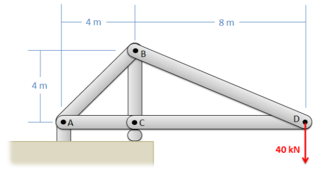
Exercise \(\PageIndex{1}\)
Use the method of joints to solve for the forces in each member of the lifting gantry truss shown below.
.png?revision=1 "homework 6 compression answers")
\(F_{AB} = 113.14\) kN T, \(F_{AC} = 80\) kN C, \(F_{BC} = 120\) kN C
\(F_{BD} = 89.44\) kN T, \(F_{CD} = 80\) kN C
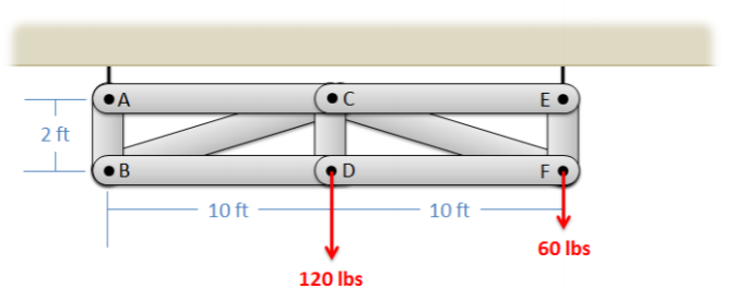
Exercise \(\PageIndex{2}\)
The truss shown below is supported by two cables at A and E, and supports two lighting rigs at D and F, as shown by the loads. Use the method of joints to determine the forces in each of the members.
.png?revision=1 "homework 6 compression answers")
\(F_{AB} = 60\) lbs T, \(F_{AC} = 0\), \(F_{BC} = 305.94\) lbs C
\(F_{BD} = 300\) lbs T, \(F_{CD} = 120\) lbs T, \(F_{CE} = 0\)
\(F_{CF} = 305.94\) lbs C, \(F_{DF} = 300\) lbs T, \(F_{EF} = 120\) lbs T
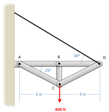
Exercise \(\PageIndex{3}\)
The truss shown below is supported by a pin joint at A, a cable at D, and is supporting a 600 N load at point C. Use the method of joints to determine the forces in each of the members. Assume the mass of the beams are negligible.
.png?revision=1 "homework 6 compression answers")
\(F_{AB} = 1162.97\) N C, \(F_{AC} = 709.86\) N T, \(F_{BC} = 0\)
\(F_{BD} = 1162.97\) N C, \(F_{CD} = 709.86\) N T
Exercise \(\PageIndex{4}\)
The space truss shown below is being used to lift a 250 lb box. The truss is anchored by a ball-and-socket joint at C (which can exert reaction forces in the \(x\), \(y\), and \(z\) directions) and supports at A and B that only exert reaction forces in the y direction. Use the method of joints to determine the forces acting all members of the truss.
.png?revision=1 "homework 6 compression answers")
\(F_{AB} = 0\), \(F_{AC} = 144.33\) lbs T, \(F_{AD} = 204.09\) lbs C
\(F_{BC} = 144.33\) lbs T, \(F_{BD} = 204.09\) lbs C, \(F_{CD} = 288.68\) lbs T
Exercise \(\PageIndex{5}\)
Use the method of sections to solve for the forces acting on members CE, CF, and DF of the gantry truss shown below.
\(F_{CE} = 0\), \(F_{CF} = 306.2\) lbs C, \(F_{DF} = 300.2\) lbs T
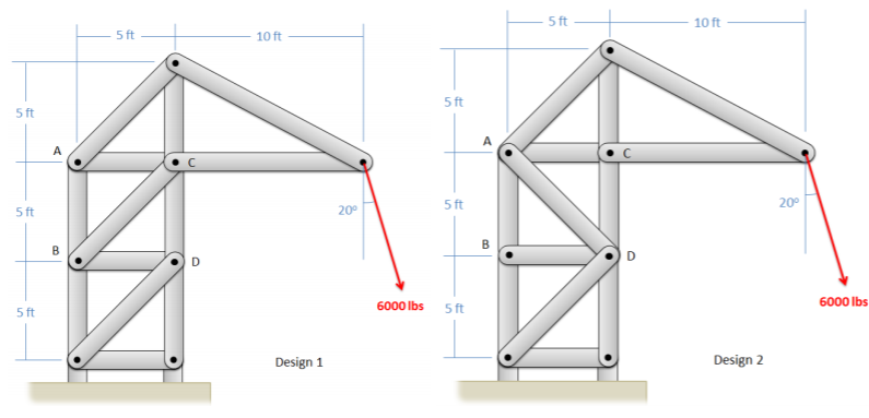
Exercise \(\PageIndex{6}\)
You are asked to compare two crane truss designs as shown below. Find the forces in members AB, BC, and CD for Design 1 and find forces AB, AD, and CD for Design 2. What member is subjected to the highest loads in either case?
.png?revision=1 "homework 6 compression answers")
Design 1: \(F_{AB} = 11,276\) lbs T, \(F_{BC} = 2902\) lbs T, \(F_{CD} = 18,967\) lbs C
Design 2: \(F_{AB} = 13,322\) lbs T, \(F_{AD} = 2902\) lbs C, \(F_{CD} = 16,914\) lbs C
The largest forces are in member CD for both designs.
Exercise \(\PageIndex{7}\)
The K truss shown below supports three loads. Assume only vertical reaction forces at the supports. Use the method of sections to determine the forces in members AB and FG. (Hint: you will need to cut through more than three members, but you can use your moment equations strategically to solve for exactly what you need).
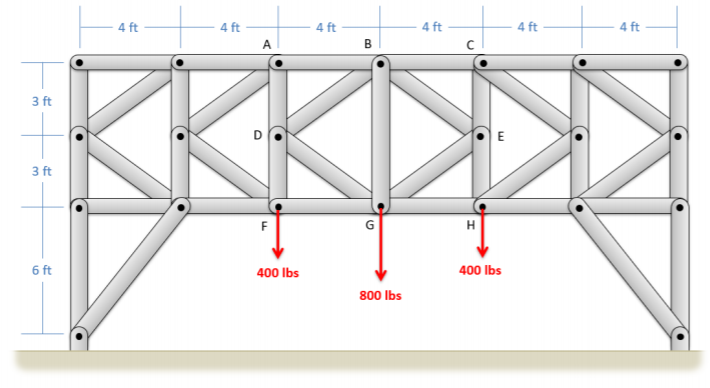.png?revision=1 "homework 6 compression answers")
\(F_{AB} = 1066.67\) lbs C, \(F_{FG} = 1066.67\) lbs T
Exercise \(\PageIndex{8}\)
The truss shown below is supported by a pin support at A and a roller support at B. Use the hybrid method of sections and joints to determine the forces in members CE, CF, and CD.
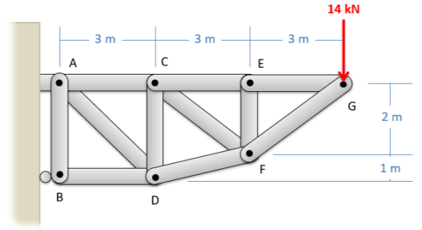.png?revision=1 "homework 6 compression answers")
\(F_{CE} = 21\) kN T, \(F_{CF} = 8.41\) kN T, \(F_{CD} = 4.67\) kN C
Exercise \(\PageIndex{9}\)
The shelf shown below is used to support a 50-lb weight. Determine the forces on members ACD and BC in the structure. Draw those forces on diagrams of each member.
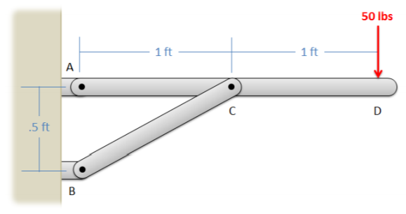.png?revision=1 "homework 6 compression answers")
\(F_{BC} = 223.6\) lbs (Compression), \(F_{A_X} = -200\) lbs, \(F_{A_Y} = -50\) lbs
Exercise \(\PageIndex{10}\)
A 20 N force is applied to a can-crushing mechanism as shown below. If the distance between points C and D is 0.1 meters, what are the forces being applied to the can at points B and D? (Hint: treat the can as a two-force member)
.png?revision=1 "homework 6 compression answers")
\(F_{can} = 148.9\) N (Compression)
Exercise \(\PageIndex{11}\)
The suspension system on a car is shown below. Assuming the wheel is supporting a load of 3300 N and assuming the system is in equilibrium, what is the force we would expect in the shock absorber (member AE)? You can assume all connections are pin joints.
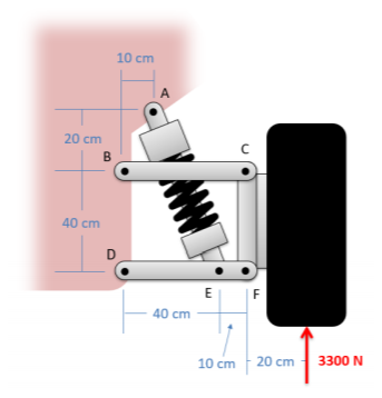.png?revision=1 "homework 6 compression answers")
\(F_{AE} = 4611.9\) N (Compression)
Exercise \(\PageIndex{12}\)
The chair shown below is subjected to forces at A and B by a person sitting in the chair. Assuming that normal forces exist at F and G, and that friction forces only act at point G (not at F), determine all the forces acting on each of the three members in the chair. Draw these forces acting on each part of the chair on a diagram.
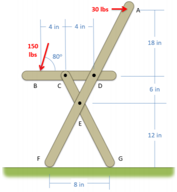.png?revision=1 "homework 6 compression answers")
\(F_F = 108.3\) lbs, \(F_{G_X} = -3.95\) lbs, \(F_{G_Y} = 39.5\) lbs
\(F_{C_X} = \pm \, 16.89\) lbs, \(F_{C_Y} = \pm \, 295.4\) lbs
\(F_{D_X} = \pm \, 142.9\) lbs, \(F_{D_Y} = \pm \, 147.7\) lbs
\(F_{E_X} = \pm \, 112.9\) lbs, \(F_{E_Y} = \pm \, 256.0\) lbs
IMAGES
VIDEO
COMMENTS
Mechanical Engineering questions and answers; HW7.6. Spring compression due to a block sliding down an inclineA point mass m=8kg is at rest on a frictionless incline angled at θ=31°. A spring of stiffness k=256Nm is placed along the incline at the bottom. The mass is at a height h=5m from the end of the spring, as shown.
This document provides instructions for Homework 6 on data compression. It asks the student to: 1) Explain why you would compress photograph files before emailing them and which form of compression (lossy or lossless) would be best for transmitting a draft manuscript or video recording. 2) Apply a lossless encoding algorithm to sample image data and report the result. 3) Identify if the ...
Brainly is the knowledge-sharing community where hundreds of millions of students and experts put their heads together to crack their toughest homework questions. Brainly - Learning, Your Way. - Homework Help, AI Tutor & Test Prep
How To: Given a function, graph its vertical stretch. Identify the value of a a. Multiply all range values by a a. If a > 1 a > 1, the graph is stretched by a factor of a a. If 0 < a< 1 0 < a < 1, the graph is compressed by a factor of a a. If a < 0 a < 0, the graph is either stretched or compressed and also reflected about the x x -axis.
7.6 Solving Systems with Gaussian Elimination; ... Yes. Sample answer: Let f (x) ... A horizontal compression results when a constant greater than 1 is multiplied by the input. A vertical compression results when a constant between 0 and 1 is multiplied by the output. 5.
CS 115 - Hw 6 Image Compression Ultimately, all data in a computer is represented with 0's and 1's. We've explored how symbols can be represented as sequences of 0's and 1's; In this problem we'll explore the representation of images using 0's and 1's. Let's begin by considering just 8-by-8 black-and-white images such as the one below: Each cell in the image is called a "pixel".
Lesson 6 Compression; Lesson 7 Assessment; There are 6 worksheets, 6 homework tasks, and an assessment test, each with answers included in this unit. How to order. 1. Add individual units to a draft order or download a blank order form below to complete manually. 2. Using a draft order you can either: Save your order online (registration or log ...
This page titled 5.8: Chapter 5 Homework Problems is shared under a CC BY-SA 4.0 license and was authored, remixed, and/or curated by Jacob Moore & Contributors ( Mechanics Map) via source content that was edited to the style and standards of the LibreTexts platform; a detailed edit history is available upon request.
Enhanced with AI, our expert help has broken down your problem into an easy-to-learn solution you can count on. Get my answer. Question: You are providing compressions on a 6 -month-old who weighs 17 pounds. Which compression depth is appropriate for this patient?
Study with Quizlet and memorize flashcards containing terms like vertical stretch, vertical compression, fraction and more.
Round to 4 decimal places. I'm almost positive I'm solving this correctly but it is wrong according to my online quiz. F (x) = k * x where k is spring constant and x is distance compressed from natural length. -6 lb = k * -18 in (Natural length of 2 ft = 24 inches. 24 - 6 in = 18. Negative for compression.) k = 1/3 lb/in. F (x) = k* x = 1/3x ...
and get 20 download points. Be the first to review this document. Partial preview of the text. ECE 537 Digital Image Processing Homework Assignment #6, Image Compression I with some answers Prof. Hintz March 28, 2008 Due: April 2, 2008 1. Can variable-length coding procedures be used to compress a histogram equalized image with 2n intensity levels?
the MPEG close MPEG Moving Picture Experts Group - Layer 4 - a standard video file format using lossy compression. file format compresses audio and video, making it more suitable for streaming media
Data Representation Homework 4 Images Answers - Free download as Word Doc (.doc / .docx), PDF File (.pdf), Text File (.txt) or read online for free. 1) A pixel is the smallest element of an image, and 8 bits are required for 256 colors. 2) File size is affected by color depth, image resolution, and dimensions in pixels. 3) Image B would have a larger file size than Image A due to having more ...
Lesson 6: Images; Download sample lesson above; Lesson 7: Data storage and compression; Assessment; There are 7 worksheets, 7 homework tasks, and an assessment test, each with answers included in this unit. How to order. 1. Add individual units to a draft order or download a blank order form below to complete manually. 2. Using a draft order ...
Mechanical Engineering. Mechanical Engineering questions and answers. 7. [5 Pts] (Textbook 6.24) Compression and heat transfer bring carbon dioxide in a piston/cylinder from 1400 kPa,20∘C to saturated vapor in an isothermal process. What are the specific heat transfer and the specific work?
To achieve a horizontal compression of the function y = 1 x by a factor of 6, we multiply the x-values by 6... View the full answer Step 2. Unlock. Step 3. Unlock. Answer. Unlock. Previous question Next question.
Homework 4: Negative Exponents Your answer should contain positive exponents only! Directions: Simplify the following monomials. 10. (2r4)-5 13. -20 20 32r 2. 5. 8. 5x2y-3 5x2 y-20 20 20 ... Homework 6: Scientific Notation XIÒI Convert the following from standard form to scientific notation. 5. 0.00000000718 3. 36.41 6. 0.0673 (o. 73
Name: Date: Unit 6: Trigonometric Identities & Equations Homework 6: Product-Sum and Power-Reducing Identities ** This is a 2-page document! ** Directions: Rewrite each expression as a sum or difference. 1. cos2y.sin5y [sin 5B)) sin - ± sin + 2 Sin 33 2. 5cos69.cos9 = 502 -e) + — Ccos 59 cos -le] cos 59 Directions: Find the exact value of ...
35) '-t -3E) a-I 1b - + wasm Agebta). Name: Unit 6: Radical Functons Homæork 7: Graphing Radial Functions ** This a 2-page document ** For quætions 1-2: Describe the bansformaäons from the parent function. strdch 21 x-axis , 3. The square root parent funcöon is translated so that it has an endpoint located at (4, -1), then vertically ...
Here's the best way to solve it. Fundamental Problem 6.6 Part A Determine the force in member AB, and state if the member is in tension or compression Suppose that P 390 lb. (Figure 1) Express your answer to three significant figures and include the appropriate units. Enter negative value in the case of compression and positive value in the ...
Our expert help has broken down your problem into an easy-to-learn solution you can count on. See Answer See Answer See Answer done loading Question: Which results only in a horizontal compression of y=(1)/(x) by a factor of 6 ? y=(1)/(6x) y=-(1)/(6x)