research paper using stratified sampling

• Research article
• Open access
• Published: 10 November 2020

Area based stratified random sampling using geospatial technology in a community-based survey

• Carrie R. Howell   ORCID: orcid.org/0000-0002-6554-6237 1 ,
• Ariann F. Nassel 2 ,
• April A. Agne 1 &
• Andrea L. Cherrington 1  

BMC Public Health volume  20 , Article number:  1678 ( 2020 ) Cite this article

28k Accesses

19 Citations

Metrics details

Most studies among Hispanics have focused on individual risk factors of obesity, with less attention on interpersonal, community and environmental determinants. Conducting community based surveys to study these determinants must ensure representativeness of disparate populations. We describe the use of a novel Geographic Information System (GIS)-based population based sampling to minimize selection bias in a rural community based study.

We conducted a community based survey to collect and examine social determinants of health and their association with obesity prevalence among a sample of Hispanics and non-Hispanic whites living in a rural community in the Southeastern United States. To ensure a balanced sample of both ethnic groups, we designed an area stratified random sampling procedure involving three stages: (1) division of the sampling area into non-overlapping strata based on Hispanic household proportion using GIS software; (2) random selection of the designated number of Census blocks from each stratum; and (3) random selection of the designated number of housing units (i.e., survey participants) from each Census block.

The proposed sample included 109 Hispanic and 107 non-Hispanic participants to be recruited from 44 Census blocks. The final sample included 106 Hispanic and 111 non-Hispanic participants. The proportion of Hispanic surveys completed per strata matched our proposed distribution: 7% for strata 1, 30% for strata 2, 58% for strata 3 and 83% for strata 4.

Utilizing a standardized area based randomized sampling approach allowed us to successfully recruit an ethnically balanced sample while conducting door to door surveys in a rural, community based study. The integration of area based randomized sampling using tools such as GIS in future community-based research should be considered, particularly when trying to reach disparate populations.

Peer Review reports

Obesity is a leading risk factor for the development of diabetes, cardiovascular illness, cancer and other chronic conditions that cause significant morbidity and mortality as well as increased health care costs [ 1 ]. Hispanics are the largest and fastest growing racial/ethnic minority group in the United States, comprising 17.3% of the population in 2014 [ 2 ], with disproportionately high obesity rates. Among adults living in the United States in 2015, the prevalence of obesity was 47% among Hispanics compared to 38% among non-Hispanic whites [ 3 ], highlighting the need to examine factors that contribute to this increased risk. To date, most studies among Hispanics have focused on individual risk factors of obesity, with less attention on interpersonal, community and environmental determinants. In order to conduct community level surveys to collect this type of data, it is crucial to ensure representativeness of both Hispanic and non-Hispanic populations in the study sample. Here we describe the use of a novel GIS-based population based sampling approach to minimize selection bias in a community based study.

Sampling for cross-sectional survey studies can be probability based or non-probability based. Probability based (e.g. random sampling) requires a defined population, where each possible unit has a known possibility of being selected [ 4 ]. Non-probability sampling methods (e.g. convenience sampling) have no known inclusion probabilities [ 5 ], producing bias and unbalanced sample representation [ 6 , 7 , 8 , 9 , 10 , 11 , 12 , 13 , 14 ]. Simple random sampling can also pose a problem for studies conducting research in minority populations. This method targets the whole population of interest and often results in minority under-representation. Stratified random sampling increases sample representativeness by dividing the study population into strata based on characteristics that are of interest to the researcher [ 15 ]. Random samples are then drawn from each strata to ensure adequate sampling of all groups. This approach reduces sampling bias; allows researchers to estimate within and between strata outcomes; and improves accuracy of results [ 15 , 16 ].

Sampling design is important in large population studies with several national surveys utilizing stratified approaches to minimize bias. The US Census Bureau conducts the American Community Survey (ACS) to produce annually updated census data estimates based on geographic units (e.g. census tract and block group). The complex sampling design consists of first stratifying the US population by census block, then calculating population based sampling rates. Appropriate weights are applied in the analytical phase so that estimates represent the full population [ 17 ]. Similarly, the National Health and Nutrition Examination Survey (NHANES) employs a stratified, multistage cluster design that oversamples specific subgroups to increase precision in health outcome estimates [ 18 ]. Smaller scale community based population studies should draw upon and incorporate aspects of these rigorous sampling designs to reduce sampling error and increase precision in estimates.

In recent years, technologies such as Geographic Information System (GIS) have been used to facilitate the sampling process in community-based research. Typically, GIS software have been used for data analysis and visualization [ 19 ]; however, health researchers have begun to realize its potential in facilitating the sampling and recruitment process, particularly in rural, developing countries [ 20 , 21 , 22 ]. To aid in sampling, GIS has been used to define populations in areas without formal census data [ 21 , 22 ]; create clusters [ 22 ]; and stratify populations [ 20 ]. Area stratified random sampling methods use area units as the strata, such as census blocks, and produce samples comparable to random digit dialing recruitment approaches [ 20 , 23 , 24 ]. This method provides an innovative way to conduct community-based health survey research, particularly when the study area is small in population. Blending aspects of complex sampling design, such as those used in national surveys, with GIS methods has the potential to strengthen community based research. Here, we describe how geospatial data and Geographic Information Systems (GIS) were used to develop an area stratified random sampling protocol that ensured demographic balance in conducting a community-based, interviewer administered survey. The study’s main aim was to examine social determinants of health and their association with obesity prevalence among a sample of Hispanics and non-Hispanic whites living in a rural community in the Southeastern United States.

Participants and setting

The population of interest resided in Albertville, Alabama where researchers had previously conducted a cervical screening study aimed at Hispanic women [ 25 ]. Located in Marshall County in the northeastern side of the state, Albertville has a population of 21,160 with 64.7% non-Hispanic white and 30.2% Hispanic as of the 2010 Census [ 26 ]. The city has two zip codes and is 26 square miles with a population density of 817 per square mile. The nearest metropolitan city with a population of over 150,000 is located 38 miles away. The median yearly income of Albertville is lower than Alabama as a whole ($35,878 vs. 40,489). The Hispanic population is concentrated to approximately 17% of the households in the city (Table  1 ).

Data was collected from participants interviewed by trained research interviewers in door-to-door canvas between June and December 2013. To be included, participants had to be at least 19 years of age, not pregnant, speak English or Spanish fluently, and self-identify as non-Hispanic white or as Hispanic/Latino. Participants were compensated with a gift card for their time. All study procedures were reviewed and approved by the University of Alabama at Birmingham’s Institutional Review Board.

Area stratified random sampling for recruitment

The goal to recruit an equal number of Hispanic and non-Hispanic participants would have been difficult to achieve by employing a completely random sampling procedure across the entire city. Therefore, a stratified random sampling procedure was created based on the Center for Disease Control and Prevention’s (CDC) Community Assessment for Public Health Emergency Responses (CASPER) sampling methodology [ 27 ]. The CASPER approach was developed using cross-sectional epidemiological principles and is a form of a community needs assessment that provides a systematic approach to collecting household information on community public health status. The cluster sampling design involves two stages: selecting clusters based on household proportions and then interviewing a set random number of households in each cluster. The CDC recommends using GIS software in the selection of the sampling frame to allow users to select portions (clusters) of geographically defined areas, such as counties or cities. In addition, GIS software provides the ability to easily develop maps for community interviewers based on the selected clusters. For this reason, CASPER provides a toolbox for use in ArcGIS software to facilitate this methodology. Using this approach in our study involved three stages: (1) division of the sampling area into non-overlapping strata based on Hispanic household proportion; (2) random selection of the designated number of Census blocks from each stratum; and (3) random selection of the designated number of housing units (i.e., survey participants) from each Census block.

Stage 1: Divide the sampling area into non-overlapping strata based on Hispanic household proportion

To ensure that the interviewers would be able to reach sufficient Hispanic households, all Census blocks within Albertville were divided into four strata based on percentage of Hispanic households using GIS software. Since Albertville city boundaries and Census block boundaries do not perfectly align with each other, a centroid criterion was used to determine whether or not a Census block belonged to Albertville city. As a result, 647 Census blocks were assigned to Albertville city. Of those, only 455 blocks contained households and the other 192 blocks were non-residential. Since the Hispanic population was concentrated in a relatively small geographic area, the 455 blocks were further divided into four unbalanced strata identified by Hispanic household proportion: < 10% Hispanic households, 10–30% Hispanic, 30–50% Hispanic, and ≥ 50% Hispanic. Roughly 60% of the blocks were assigned to the ≤10% of Hispanic households stratum, with 7% ( N  = 32) of the blocks assigned to the > 50% of Hispanic households stratum (see Table  2 and Fig.  1 ).

Census blocks in Albertville, AL by Hispanic household proportion. Map of census block groups in Albertville, AL. Darker shading indicates higher Hispanic household proportions. Map developed using licensed ArcGIS software

Stage 2: Randomly select the designated number of Census blocks from each stratum

Our goal was to recruit a total of 200 participants, with a distribution of 50% Hispanic and 50% non-Hispanic white (1:1 ratio). Maps denoted that the Hispanic population was largely concentrated in small area blocks (Fig.  1 ). Although smaller blocks suggest higher population density, they also contain fewer individuals and households compared with larger blocks. Since Hispanics comprised a smaller proportion of total households (17%), we needed to oversample blocks with higher concentrations of Hispanic households in order to reach an equal number of Hispanic and Non-Hispanic surveys. For these reasons we took the following approach to determine the number of Census blocks to select from each group, and the number of housing units to select from each Census block.

Considering the varying population size across blocks, it was determined to be more feasible to plan fewer surveys per block in more Hispanic population concentrated areas (i.e., strata 3 & 4 in Table  2 ), and more surveys per block in more non-Hispanic population concentrated areas (i.e., strata 1 & 2 in Table  2 ). As a result, we selected 10 blocks with 6 surveys per block from strata 1 and 2 and 12 blocks with 4 surveys per block from strata 3 and 4. These numbers were somewhat arbitrary, balancing the concern that selecting too many blocks which would increase cost, while taking care to not plan for an unrealistic quota of surveys per block when not feasible (e.g. the smallest block in the study area contained only 8 households).

For strata 1 and 2, distribution of Hispanic versus non-Hispanic surveys within each block roughly reflected the proportions of Hispanic and non-Hispanic households in the corresponding group. Since oversampling of the Hispanic population was needed to achieve the recruitment goal, proportions of Hispanic surveys in strata 3 and 4 were set higher than the actual proportions of Hispanic households. Table  2 shows the proposed number of blocks to select from each group and numbers of Hispanic versus non-Hispanic surveys projected within each block. In total, we proposed 109 Hispanic surveys and 107 non-Hispanic surveys from 44 blocks.

Once the number of blocks from each group were determined, the CASPER toolkit developed by the CDC was utilized to generate random samples [ 27 ]. We used an add-on program developed for ArcGIS by the CDC to generate random samples using a polygon layer that represents the sampling area and non-overlapping clusters within the sampling area. In our study, the four strata were our sampling areas with Census blocks the non-overlapping clusters, accounting for the number of housing units within each cluster. The random sampling procedure was repeated four times, once for each stratum. Figure  2 shows the 44 random blocks selected from the entire study area using this approach.

Census blocks selected for recruitment. Map of the 44 census block groups randomly selected in Albertville, AL using an area stratified random sampling approach. Blue outline indicates block group selected. Map developed using licensed ArcGIS software

Stage 3: Randomly select the designated number of housing units from each Census block

Interviewers were provided with satellite maps (Fig.  3 ) for each block randomized with detailed instructions regarding how to randomly select the designated number of housing units within each block. The systematic random sampling method described in the CASPER toolkit [ 27 ] was adapted and modified to develop the study’s survey protocol:

A starting point (address) for each sampling block was provided. This was the first house for the interviewers to survey.

After completing the first survey, interviewers would walk or drive in either direction to the next N th house. This would be the next household for the interviewers to survey.

If no one answers the door, continue to the next N th house.

Continue traveling through the sampling block, selecting every N th house until they have completed the designated number of surveys for that sampling block.

If the interviewers circled back to the starting point and had not completed the designated number of surveys, they would then proceed through the block again and select every (N + 1) th house. For example, if Block A had an N of 8, in the next pass the interviewer would approach every 9th house.

Field interviewer block map. An example of the satellite image map provided to interviewers to conduct field surveys. Map data image provided by© 2013 Google; Imagery© 2013 MaxarTechnologies

The N used in the protocol was determined by dividing the total number of housing units by the designated number of surveys to complete in each block, and thus could vary from block to block. For example, if a block contained 50 housing units and the designated number of surveys was 6 for that block, the N would be 8. Values of N for each individual block were provided in the instructions to the interviewers. Additional instructions with regards to abandoned homes, businesses, duplexes and apartment complexes, multiple family homes, and trailer parks were also provided.

The proposed sample included 109 Hispanic and 107 non-Hispanic participants to be recruited from 44 Census blocks. After exhausting all 44 blocks, interviewers were unable to meet recruitment goals for the proposed number of surveys in each block. Twenty additional blocks were selected using the same random sampling procedure described above, including two from strata 1 (≤10% of Hispanic households), two from strata 2 (10–30% of Hispanic households), six from strata 3 (30–50% of Hispanic households), and ten from strata 4 (> 50% of Hispanic households). More blocks with higher Hispanic population density were selected because field interviewers found that recruitment of Hispanic participants was particularly challenging. The final sample included 106 Hispanic and 111 non-Hispanic participants. The number of surveys completed from each block ranged from 0 to 11, with an average of 3.4 surveys per block (Table  3 and Fig.  4 ).

Number of participants by Census block. Map of census block groups in Albertville, AL with the number of participants who completed a survey. Darker shading indicates more participants. Map developed using licensed ArcGIS software

Post-hoc chi-square and Fishers exact tests were used to test the proposed distribution of surveys by ethnicity status to the proportions of surveys completed. P -values > 0.05 indicate that actual proportions did not differ from proposed population based proportions. The proportion of Hispanic surveys completed per strata were similar to our proposed distribution for strata 1–3: 7% for strata 1 ( p  = 1.0), 30% for strata 2 ( p  = 0.71), and 58% for strata 3 ( p  = 0.07). Although Strata 4 (83% Hispanic surveys, p  = 0.002) had statistically different proportions, this was expected due to the need to oversample Hispanic surveys from this strata.

Here we demonstrate the successful use of a novel area stratified random sampling technique utilizing GIS that ensured ethnic balance in the recruitment of our community canvased study sample. Field recruitment in community studies presents challenges in minimizing selection bias and ensuring demographic representation. Here, integrating GIS based technology with census data provided a standardized and objective approach to recruitment to address these issues. Specifically, we utilized GIS to create and visualize non-overlapping strata to determine individual stratums and to randomly select Census blocks within those strata. Our approach ensured the 1:1 ratio of Hispanics to non-Hispanics in our study, minimized selection bias, and provided an approach that was easy for the ‘boots on the ground’ interviewers to implement. Moreover, the distribution of completed Hispanic surveys by stratum closely matched our original proposed proportions (defined based on percentage of Hispanic households in block), giving our sample geographic representation by Albertville block.

Utilizing GIS to facilitate community-based research, such as targeting areas for program planning or ensuring random sampling of survey respondents [ 28 ], has been implemented in recent population based studies. This method has been particularly useful in rural, developing countries [ 20 , 21 , 22 , 29 ]. Defar et al. used GIS methods to conduct a cross-sectional survey in Ethiopia on maternal and child health care utilization in a similar two-stage process as the current study [ 29 ] while Wampler et al. used GIS to facilitate the random selection of households in specific areas in Haiti for water quality research [ 22 ]. Akin to the results here, a study that compared simple random sampling to stratified sampling by zip code and census tract found that area based stratified sampling ensured a higher representativeness of Hispanic residents in audits of tobacco retailers in an urban area [ 30 ]. In the public health realm, Lafontaine et al. developed a spatial random sampling method to conduct neighborhood built environment audits and concluded that this approach was more cost and time effective [ 31 ]. Likewise, using the approach herein resulted in recruiting our Hispanic sample in a more efficient manner.

It is important to note that we selected the number of blocks for randomization and recruitment based on feasibility but nonetheless in an arbitrary fashion. While this resulted in a balanced sample for our study, this will likely not translate into other scenarios. Since stratification by design results in subgroups that are over or under represented compared to the overall population [ 15 ], taking the actual population weights of each census tract into account when selecting blocks would have been more appropriate. Since the ultimate goal in sampling is to select a study sample that is representative of the population, applying population sampling weights and using model-based approaches such as raking prior to analysis are essential. Raking adjusts the sampling weights by forcing the survey totals to match proportions in the known population [ 32 ].

Our approach was not without challenges or limitations. When conducting the door to door surveys, interviewers were provided with detailed protocol and satellite maps. However, multiple issues arose. First, there was a significant number of houses that provided “no answer” and we had to implement the N + 1 sampling multiple times to reach recruitment targets. Time constraints also impacted interviewers. Some blocks sampled had a count number that was large ( N  > 14), which decreased sampling efficiency as driving from one house to the next could exceed 10 min. Another limitation of the study is that we used the population and household counts from the 2010 Decennial Census data, which may have underestimated the number of Hispanics in Albertville at the time of data collection (2013). Further, the criterion used to divide the study area was Census block group and 2010 Census estimates were likely different than the true distribution of Hispanic households by block in 2013. Lastly, it is important to note that CASPER was designed for use in the United States and associated territories and uses data collected from the census bureau to create population based sampling areas and clusters. However, since CASPER was developed based on an epidemiological two-stage cluster sampling approach, it is possible to conduct this type of sampling in other countries where census type data are available using the CASPER protocol as a guide.

Overall, we developed a standardized area based randomized sampling protocol that allowed us to successful recruit an ethnically balanced sample while conducting door to door community surveys. Minimizing selection bias in community-based surveys can be difficult; however, advancement in technological tools such as GIS provides novel approaches to address these biases. Based on our results here, we advocate the integration of area based randomized sampling in future community-based research, particularly when trying to reach disparate populations.

Availability of data and materials

Data sharing is not applicable to this article as no datasets were generated or analyzed during the current study.

Abbreviations

• Geographic information systems

Community Assessment for Public Health Emergency Response

Centers for Disease Control and Prevention

American Community Survey

National Health and Nutrition Examination Study

World Health Organization. Obesity and overweight fact sheet no. 311. 2013. Available from: http://www.who.int/mediacentre/factsheets/fs311/en/index.html .

Stepler R, Brown A. 2014, Hispanics in the United States statistical portrait. 2016. Available from: https://www.pewresearch.org/hispanic/2016/04/19/2014-statistical-information-on-hispanics-in-united-states/ .

Google Scholar  

Hales CM, Carroll MD, Fryar CD, Ogden CL. Prevalence of obesity among adults and youth: United States, 2015-2016. NCHS Data Brief. 2017;(288):1–8.

Tashakkori A, Teddlie C. Handbook on mixed methods in the behavioral and social sciences. Thousand Oaks: Sage; 2003.

Doherty M. Probability versus non-probability sampling in sample surveys. N Z Stat Rev. 1994;4:21–8.

Fanzana B, Srunv E. A venue-based method for sampling hard-to-reach populations. Public Health Rep. 2001:216–22.

Klein JD, Thomas RK, Sutter EJ. Self-reported smoking in online surveys: prevalence estimate validity and item format effects. Med Care. 2007;45(7):691–5.

Article   Google Scholar  

Roster CA, Rogers RD, Albaum G, Klein D. A comparison of response characteristics from web and telephone surveys. Int J Mark Res. 2004;46(3):359–73.

Schillewaert N, Meulemeester P. Comparing response distributions of offline and online. Int J Mark Res. 2005;47(2):163–78.

Schonlau M, Zapert K, Simon LP, Sanstad KH, Marcus SM, Adams J, et al. A comparison between responses from a propensity-weighted web survey and an identical RDD survey. Soc Sci Comput Rev. 2004;22(1):128–38.

Spijkerman R, Knibbe R, Knoops K, Van De Mheen D, Van Den Eijnden R. The utility of online panel surveys versus computer assisted interviews in obtaining substance use prevalence estimates in the Netherlands. Addiction. 2009;104(10):1641–5.

Bethell C, Fiorillo J, Lansky D, Hendryx M, Knickman J. Online consumer surveys as a methodology for assessing the quality of the United States health care system. J Med Internet Res. 2004;6(1):e2.

Chang L, Krosnick JA. National surveys via RDD telephone interviewing versus the internet: comparing sample representativeness and response quality. Public Opin Q. 2009;73(4):641–78.

Malhotra N, Krosnick JA. The effect of survey mode and sampling on inferences about political attitudes and behavior: comparing the 2000 and 2004 ANES to internet surveys with nonprobability samples. Polit Anal. 2007;15(3):286–323.

Teddlie C, Yu F. Mixed methods sampling: a typology with examples. J Mixed Methods Res. 2007;1(1):77–100.

Elfil M, Negida A. Sampling methods in clinical research; an educational review. Emerg (Tehran). 2017;5(1):e52.

American Community Survey Design and Methodology. Chapter 4: Sample design and selection. 2014. https://www2.census.gov/programs-surveys/acs/methodology/design_and_methodology/acs_design_methodology_ch04_2014.pdf?# . Accessed 20 July 2020.

National Health and Nutrition Examination Survey, 2015−2018: Sample Design and Estimation Procedures. https://www.cdc.gov/nchs/data/series/sr_02/sr02-184-508.pdf . Accessed 20 July 2020.

Cromley EK, McLafferty SL. GIS and public health: Guilford Press; 2011.

Kondo MC, Bream KD, Barg FK, Branas CC. A random spatial sampling method in a rural developing nation. BMC Public Health. 2014;14:338.

Lin Y, Kuwayama DP. Using satellite imagery and GPS technology to create random sampling frames in high risk environments. Int J Surg. 2016;32:123–8.

Wampler PJ, Rediske RR, Molla AR. Using ArcMap, Google Earth, and Global Positioning Systems to select and locate random households in rural Haiti. Int J Health Geogr. 2013;12:3.

Aquilino WS, Wright DL. Substance use estimates from RDD and area probability samples: impact of differential screening methods and unit nonresponse. Public Opin Q. 1996;60(4):563–73.

Lete C, Holly EA, Roseman DS, Thomas DB. Comparison of control subjects recruited by random digit dialing and area survey. Am J Epidemiol. 1994;140(7):643–8.

Scarinci IC, Garces-Palacio IC, Morales-Aleman MM, McGuire A. Sowing the seeds of health: training of community health advisors to promote breast and cervical cancer screening among Latina immigrants in Alabama. J Health Care Poor Underserved. 2016;27(4):1779–93.

US Census Bureau. QuickFacts: Albertville, AL. https://www.census.gov/quickfacts/fact/table/albertvillecityalabama/PST045218 .

Centers for Disease Control and Prevention. Community Assessment for Public Health Emergency Response (CASPER), sampling methodology. https://www.cdc.gov/nceh/casper/sampling-methodology.htm .

Quon Huber MS, Van Egeren LA, Pierce SJ, Foster-Fishman PG. GIS applications for community-based research and action: mapping change in a community-building initiative. J Prev Interv Community. 2009;37(1):5–20.

Defar A, Okwaraji YB, Tigabu Z, Persson LA, Alemu K. Geographic differences in maternal and child health care utilization in four Ethiopian regions; a cross-sectional study. Int J Equity Health. 2019;18(1):173.

Lee JGL, Shook-Sa BE, Bowling JM, Ribisl KM. Comparison of sampling strategies for tobacco retailer inspections to maximize coverage in vulnerable areas and minimize cost. Nicotine Tob Res. 2018;20(11):1353–8.

Lafontaine SJ, Sawada M, Kristjansson E. A direct observation method for auditing large urban centers using stratified sampling, mobile GIS technology and virtual environments. Int J Health Geogr. 2017;16(1):6.

Battaglia MP, Izrael D, Hoaglin DC, Frankel MR. Practical considerations in raking survey data. Surv Pract. 2009;2(5):1–10.

Download references

Acknowledgements

We especially thank Matthew Carle, Morgan Griesemer Lepard, Ynhi Thai, Meghan Meehan, Amancia Carrera, Sylvia Alavarez Mancinas, Susan Henry Barber, and Chris Caudill for their tireless efforts to canvas neighborhoods and interviews participants. We would also like to thank all our participants, the office of the Mayor of Albertville, the Albertville Police Department, support staff, and others who helped make this study possible.

This work was supported by grants from the University of Alabama with funding from the National Institute of Minority Health and Health Disparities (U54MD008176) and support from the National Institutes of Health, National Institute of Diabetes and Digestive and Kidney Diseases, UAB Diabetes Research Center [1P60DK079626–01]. The content is solely the responsibility of the authors and does not necessarily represent the official views of the National Institute of Minority Health and Health or National Institute of Diabetes and Digestive and Kidney Diseases or the National Institutes of Health or others supporting this work. All sources of funding had no role in study design; collection, analysis, and interpretation of data; writing the report; or the decision to submit the report for publication.

Author information

Authors and affiliations.

Department of Medicine, Division of Preventive Medicine, University of Alabama at Birmingham, Medical Towers 62, 1717 11th Avenue South, Birmingham, AL, 35205, USA

Carrie R. Howell, April A. Agne & Andrea L. Cherrington

School of Public Health, University of Alabama at Birmingham, 1665 University Blvd, Birmingham, AL, 35233, USA

Wei Su & Ariann F. Nassel

You can also search for this author in PubMed   Google Scholar

Contributions

WS, AC made substantial contributions to the design of the work. CH, WS, AC made substantial contributions to the analysis, interpretation of data and drafted the work. AN and AA made substantial contributions to the acquisition and interpretation of data. All authors read and approved the final manuscript and are accountable for the accuracy and integrity of the work presented.

Corresponding author

Correspondence to Carrie R. Howell .

Ethics declarations

Ethics approval and consent to participate.

This study was approved by the University of Alabama at Birmingham Institutional Review board and documented written informed consent was obtained from all participants prior to participation.

Consent for publication

Not applicable.

Competing interests

The authors declare they have no competing interests or financial relationships relevant to this article to disclose.

Additional information

Publisher’s note.

Springer Nature remains neutral with regard to jurisdictional claims in published maps and institutional affiliations.

Rights and permissions

Open Access This article is licensed under a Creative Commons Attribution 4.0 International License, which permits use, sharing, adaptation, distribution and reproduction in any medium or format, as long as you give appropriate credit to the original author(s) and the source, provide a link to the Creative Commons licence, and indicate if changes were made. The images or other third party material in this article are included in the article's Creative Commons licence, unless indicated otherwise in a credit line to the material. If material is not included in the article's Creative Commons licence and your intended use is not permitted by statutory regulation or exceeds the permitted use, you will need to obtain permission directly from the copyright holder. To view a copy of this licence, visit http://creativecommons.org/licenses/by/4.0/ . The Creative Commons Public Domain Dedication waiver ( http://creativecommons.org/publicdomain/zero/1.0/ ) applies to the data made available in this article, unless otherwise stated in a credit line to the data.

Reprints and permissions

About this article

Cite this article.

Howell, C.R., Su, W., Nassel, A.F. et al. Area based stratified random sampling using geospatial technology in a community-based survey. BMC Public Health 20 , 1678 (2020). https://doi.org/10.1186/s12889-020-09793-0

Download citation

Received : 22 May 2020

Accepted : 29 October 2020

Published : 10 November 2020

DOI : https://doi.org/10.1186/s12889-020-09793-0

Share this article

Anyone you share the following link with will be able to read this content:

Sorry, a shareable link is not currently available for this article.

Provided by the Springer Nature SharedIt content-sharing initiative

• Stratified random sampling
• Hispanic population
• Rural population
• Community based methods

BMC Public Health

ISSN: 1471-2458

• Submission enquiries: [email protected]
• General enquiries: [email protected]

Have a language expert improve your writing

Run a free plagiarism check in 10 minutes, automatically generate references for free.

• Knowledge Base
• Methodology

Stratified Sampling | A Step-by-Step Guide with Examples

Published on 3 May 2022 by Lauren Thomas .

In a stratified sample , researchers divide a population into homogeneous subpopulations called strata (the plural of stratum) based on specific characteristics (e.g., race, gender identity, location). Every member of the population studied should be in exactly one stratum.

Each stratum is then sampled using another probability sampling method, such as cluster or simple random sampling, allowing researchers to estimate statistical measures for each subpopulation.

Researchers rely on stratified sampling when a population’s characteristics are diverse and they want to ensure that every characteristic is properly represented in the sample.

Table of contents

When to use stratified sampling, step 1: define your population and subgroups, step 2: separate the population into strata, step 3: decide on the sample size for each stratum, step 4: randomly sample from each stratum, frequently asked questions about stratified sampling.

To use stratified sampling, you need to be able to divide your population into mutually exclusive and exhaustive subgroups. That means every member of the population can be clearly classified into exactly one subgroup.

Stratified sampling is the best choice among the probability sampling methods when you believe that subgroups will have different mean values for the variable(s) you’re studying. It has several potential advantages:

Ensuring the diversity of your sample

A stratified sample includes subjects from every subgroup, ensuring that it reflects the diversity of your population. It is theoretically possible (albeit unlikely) that this would not happen when using other sampling methods such as simple random sampling .

Ensuring similar variance

If you want the data collected from each subgroup to have a similar level of variance , you need a similar sample size for each subgroup.

With other methods of sampling, you might end up with a low sample size for certain subgroups because they’re less common in the overall population.

Lowering the overall variance in the population

Although your overall population can be quite heterogeneous, it may be more homogenous within certain subgroups.

For example, if you are studying how a new schooling program affects the test scores of children, both their original scores and any change in scores will most likely be highly correlated with family income. The scores are likely to be grouped by family income category.

In this case, stratified sampling allows for more precise measures of the variables you wish to study, with lower variance within each subgroup and therefore for the population as a whole.

Allowing for a variety of data collection methods

Sometimes you may need to use different methods to collect data from different subgroups.

For example, in order to lower the cost and difficulty of your study, you may want to sample urban subjects by going door to door, but rural subjects by post.

Because only a small proportion of this university’s graduates have obtained a doctoral degree, using a simple random sample would likely give you a sample size too small to properly compare the differences between men, women, and those who do not identify as men or women with a doctoral degree vs those without one.

Prevent plagiarism, run a free check.

As with other methods of probability sampling , you should begin by clearly defining the population from which your sample will be taken.

Choosing characteristics for stratification

You must also choose the characteristic that you will use to divide your groups. This choice is very important: since each member of the population can only be placed in only one subgroup, the classification of each subject to each subgroup should be clear and obvious.

Stratifying by multiple characteristics

You can choose to stratify by multiple different characteristics at once, so long as you can clearly match every subject to exactly one subgroup. In this case, to get the total number of subgroups, you multiply the numbers of strata for each characteristic.

For instance, if you were stratifying by both race and gender identity, using four groups for the former and three for the latter, you would have 4 × 3 = 12 groups in total.

Next, collect a list of every member of the population, and assign each member to a stratum.

You must ensure that each stratum is mutually exclusive (there is no overlap between them), but that together, they contain the entire population.

Combining these characteristics, you have nine groups in total. Each graduate must be assigned to exactly one group.

First, you need to decide whether you want your sample to be proportionate or disproportionate.

Proportionate vs disproportionate sampling

In proportionate sampling, the sample size of each stratum is equal to the subgroup’s proportion in the population as a whole.

Subgroups that are less represented in the greater population (for example, rural populations, which make up a lower portion of the population in most countries) will also be less represented in the sample.

In disproportionate sampling, the sample sizes of each strata are disproportionate to their representation in the population as a whole.

You might choose this method if you wish to study a particularly underrepresented subgroup whose sample size would otherwise be too low to allow you to draw any statistical conclusions.

Sample size

Next, you can decide on your total sample size. This should be large enough to ensure you can draw statistical conclusions about each subgroup.

If you know your desired margin of error and confidence level as well as estimated size and standard deviation of the population you are working with, you can use a sample size calculator to estimate the necessary numbers.

Finally, you should use another probability sampling method , such as simple random or systematic sampling , to sample from within each stratum.

If properly done, the randomisation inherent in such methods will allow you to obtain a sample that is representative of that particular subgroup.

In stratified sampling , researchers divide subjects into subgroups called strata based on characteristics that they share (e.g., race, gender, educational attainment).

Once divided, each subgroup is randomly sampled using another probability sampling method .

You should use stratified sampling when your sample can be divided into mutually exclusive and exhaustive subgroups that you believe will take on different mean values for the variable that you’re studying.

Using stratified sampling will allow you to obtain more precise (with lower variance ) statistical estimates of whatever you are trying to measure.

For example, say you want to investigate how income differs based on educational attainment, but you know that this relationship can vary based on race. Using stratified sampling, you can ensure you obtain a large enough sample from each racial group, allowing you to draw more precise conclusions.

Yes, you can create a stratified sample using multiple characteristics, but you must ensure that every participant in your study belongs to one and only one subgroup. In this case, you multiply the numbers of subgroups for each characteristic to get the total number of groups.

For example, if you were stratifying by location with three subgroups (urban, rural, or suburban) and marital status with five subgroups (single, divorced, widowed, married, or partnered), you would have 3 × 5 = 15 subgroups.

Probability sampling means that every member of the target population has a known chance of being included in the sample.

Probability sampling methods include simple random sampling , systematic sampling , stratified sampling , and cluster sampling .

Cite this Scribbr article

If you want to cite this source, you can copy and paste the citation or click the ‘Cite this Scribbr article’ button to automatically add the citation to our free Reference Generator.

Thomas, L. (2022, May 03). Stratified Sampling | A Step-by-Step Guide with Examples. Scribbr. Retrieved 6 May 2024, from https://www.scribbr.co.uk/research-methods/stratified-sampling-method/

Is this article helpful?

Lauren Thomas

Other students also liked, sampling methods | types, techniques, & examples, cluster sampling | a simple step-by-step guide with examples, simple random sampling | definition, steps & examples.

Click through the PLOS taxonomy to find articles in your field.

For more information about PLOS Subject Areas, click here .

Loading metrics

Open Access

Peer-reviewed

Research Article

Stratified Sampling of Neighborhood Sections for Population Estimation: A Case Study of Bo City, Sierra Leone

Independent consultant, Fairfax, Virginia, United States of America

Affiliation Information Technology Division, Naval Research Laboratory, Washington, District of Columbia, United States of America

Affiliation Department of Global and Community Health, George Mason University, Fairfax, Virginia, United States of America

Affiliations Njala University, Bo, Sierra Leone, Mercy Hospital Research Laboratory, Bo, Sierra Leone

Affiliation Mercy Hospital Research Laboratory, Bo, Sierra Leone

* E-mail: [email protected]

Affiliation Center for Bio/Molecular Science and Engineering, Naval Research Laboratory, Washington, District of Columbia, United States of America

• Roger Hillson, 
• Joel D. Alejandre, 
• Kathryn H. Jacobsen, 
• Rashid Ansumana, 
• Alfred S. Bockarie, 
• Umaru Bangura, 
• Joseph M. Lamin, 
• David A. Stenger

• Published: July 15, 2015
• https://doi.org/10.1371/journal.pone.0132850
• Reader Comments

There is a need for better estimators of population size in places that have undergone rapid growth and where collection of census data is difficult. We explored simulated estimates of urban population based on survey data from Bo, Sierra Leone, using two approaches: (1) stratified sampling from across 20 neighborhoods and (2) stratified single-stage cluster sampling of only four randomly-sampled neighborhoods. The stratification variables evaluated were (a) occupants per individual residence, (b) occupants per neighborhood, and (c) residential structures per neighborhood. For method (1), stratification variable (a) yielded the most accurate re-estimate of the current total population. Stratification variable (c), which can be estimated from aerial photography and zoning type verification, and variable (b), which could be ascertained by surveying a limited number of households, increased the accuracy of method (2). Small household-level surveys with appropriate sampling methods can yield reasonably accurate estimations of urban populations.

Citation: Hillson R, Alejandre JD, Jacobsen KH, Ansumana R, Bockarie AS, Bangura U, et al. (2015) Stratified Sampling of Neighborhood Sections for Population Estimation: A Case Study of Bo City, Sierra Leone. PLoS ONE 10(7): e0132850. https://doi.org/10.1371/journal.pone.0132850

Editor: Maciej F. Boni, University of Oxford, VIET NAM

Received: February 2, 2015; Accepted: June 19, 2015; Published: July 15, 2015

This is an open access article, free of all copyright, and may be freely reproduced, distributed, transmitted, modified, built upon, or otherwise used by anyone for any lawful purpose. The work is made available under the Creative Commons CC0 public domain dedication

Data Availability: All relevant tabular data are within the paper and its Supporting Information files. GIS data are available on OpenStreetMap ( http://osm.org/go/am_ZKeeU- ).

Funding: This work was funded by the Defense Threat Reduction Agency, Joint Science and Technology Office ( http://www.dvidshub.net/unit/DTRA-CB#.UoUqZ9wo5zk ) via contract to myself at the Naval Research Laboratory. A subcontract from NRL with George Mason University was used to provide support for contractors (Rashid Ansumana, Alfred Bockarie, Umaru Bangura and Joseph Lamin) working at Mercy Hospital Research Laboratory in Bo, Sierra Leone. There is no past, present or future Intellectual Property associated with the work described in the paper, and none of the authors have any financial interests or conflicts in the outcome of the study. The funders had no role in study design, data collection and analysis, decision to publish, or preparation of the manuscript.

Competing interests: The authors have declared that no competing interests exist.

Introduction

The population of a region of interest must be estimated if one’s goal is to convert incidence counts into rates. This conversion is not always necessary, because some epidemiological parameters can now be estimated from incidence counts alone, including the interval between successive cases, and the reproductive number R 0 , which is the average number of secondary cases attributable to a primary cause [ 1 , 2 ]. If these parameters are insufficient to evaluate the models, it may be necessary to calculate the total population N . The 5 brief examples that follow illustrate both the necessity of doing so, and some of the difficulties that may be encountered.

In resource-limited environments, it may be possible to use both aerial imagery and limited residential survey data to estimate the population of a region of interest, as shown in the first two examples. Using ground truth data for the measured population of 20 sections in Bo City, Sierra Leone, we compared the uncertainty of estimating the population using survey data for either (1) occupants per residence or (2) rooftop area per resident. The latter variable was computed by manually digitizing the rooftop areas of residential structures in 5 sections of Bo, and calculating the ratio of rooftop area per occupant for each residence [ 3 ]. The ability to rapidly estimate the population of both temporary and unplanned settlements is critical for planning resource allocation for refugee and internally displaced populations as well as for places undergoing rapid unplanned urbanization, since in these settings there is usually not a stable residential population. Checchi et al. [ 4 ] have developed a two-step method for estimating a refugee population that requires (1) estimating the number of temporary residential structures from satellite imagery and (2) estimating the mean occupancy per structure. The product of the estimate (1) “number of structures” and (2) “mean number of persons per structure” yields an estimate of the total refugee population.

As shown in the next 2 examples, if salient population data are available either directly or by interpolation; derived rates of infection, immunity, or morbidity may be calculated. The standard SEIR (Susceptible, Exposed, Infectious, Recovered) compartmental epidemiological model [ 5 , 6 ] requires N as a parameter. Glasser et al. [ 6 ] simulated the implementation of two different influenza vaccination policies, in order to predict their effect on both the incidence of infection and the rate of morbidity. They applied a SEIR model parameterized by demographic parameters for the United States (2005), including the total population stratified by age. The age-specific death rates attributable to pneumonia and influenza were estimated, as were the death rates from all other remaining causes. Gomez-Elipe et al. [ 7 ] have developed a model for forecasting the incidence of Malaria in Karuzi, Burundi (1997–2003). To convert the reported instances of malaria to a rate, the investigators divided the rate by the 2006 population census, after rescaling (decrementing) by the population growth factors for the intervals from 1995–2000 (growth factor = 1.32) and 2000–2005 (growth factor = 3.29).

In demographically-diverse environments, different methods may be required to estimate the population at different locations, as shown in our final example. The GRUMPv1 (Global Rural-Urban Mapping Project, Version One) , separates the urban population density estimates from the population of the surrounding areas. In addition to enumerated city population data, city footprints can be established by analyzing nighttime satellite images, but this approach may fail to capture small informal settlements in Africa and rural Asia [ 8 ] (page 9). Accordingly, several corrections are applied for poorly illuminated settlements [ 8 ] (page 9), and point estimates are provided for settlement populations exceeding 1,000. Many models utilize GRUMP for epidemiological modeling, including [ 8 , 9 ].

Proposed analysis

In a previous study [ 3 ], a Finite Population Bootstrap (FPB) [ 10 ] (page 92) was used to compare the relative uncertainty of two population estimators: an occupancy-based estimator and a rooftop area-based estimator. For the region of interest, the former was estimated as the product of (1) the average number of persons per residential structure multiplied by (2) the total number of residential structures; and the latter was calculated as (1) the average number of persons per rooftop area (i.e., persons per m 2 ) multiplied by (2) the total estimated rooftop area in m 2 . Both estimators were effective, but the uncertainty was about 20% less for the occupancy-based estimator [ 3 ] (page 10). Both the occupancy-based and rooftop area-based population estimators were evaluated by simulating simple random sampling without replacement (SRSWOR).

The analysis in this current paper will evaluate the use of stratified sampling for population estimation, and will demonstrate the reduction in the uncertainty of the population estimate achievable relative to SRSWOR. Two different stratification designs will be explored: (1) optimal stratification by “persons per structure” and (2) stratified single-stage cluster sampling. The relative advantages and restrictions of both methods will be discussed. The city of Bo itself is approximately 30.1 km 2 in area, and is divided into 68 uniquely-shaped neighborhoods or sections [ 11 ](see Fig 1 in [ 3 ] and Table 1 ). These sections vary in size from 0.02 km 2 (Toubu) to 2.33 km 2 (Bo Government Reservation). For 20 of the 68 sections, residential survey data are also available [ 3 ] (see Table 1 ). The ground truth survey data for these 20 sections will provide the basis for simulated sampling using different stratification protocols, and for quantifying the reduction in the uncertainty of the population estimate achievable.

• PPT PowerPoint slide
• PNG larger image
• TIFF original image

https://doi.org/10.1371/journal.pone.0132850.t001

The first approach, optimal stratification by persons per structure, requires that the number of persons per structure be already known for all residential structures; possibly from a prior survey or census data. The objective is to exploit this prior data to design an improved stratification protocol for re-estimating the population, and to demonstrate a significant reduction in the uncertainty of the population estimate relative to random sampling. Single-stage cluster sampling is useful if the number of sections that can actually be sampled is restricted, perhaps because of cost or schedule limitations. In our examples, the simulated cluster sampling will be restricted to 4 of the 20 available sections. We will investigate the reduction in uncertainty that can be achieved by using a stratified cluster sampling protocol, rather than random selection, to select the 4 sections on each simulation trial. Each section will be completely sampled.

Note that choice of population estimators is independent of the stratified sampling protocol selected for simulated data collection. A stratified Horvitz-Thompson [ 12 ] population estimator will be evaluated for all examples. We have also extended our original FPB model to support stratified sampling [ 10 ], and partial results from the latter will be contrasted with estimates obtained using the stratified Horvitz-Thompson estimator. Neither the stratified FPB nor the Horvitz-Thompson estimator were used in the prior study.

• What reduction in the uncertainty of the population estimate can be achieved by stratified sampling—relative to simple random sampling of all sections—if the residential survey records are first partitioned into mutually-exclusive strata with non-overlapping ranges of “persons per residential structure?”
• Can any reduction in uncertainty be achieved—again relative to simple random sampling of all sections—if the sections are partitioned into mutually-exclusive and exhaustive strata, rather than partitioning the individual records (PSUs) into strata?
• For single-stage cluster sampling, if the sections (clusters) are partitioned into mutually-exclusive strata by “total residential structures per section,” what is the relative reduction in uncertainty that can achieved using stratified cluster sampling, rather than unclassified cluster sampling?
• Does stratification by the “total persons per section”—if known—further reduce the uncertainty of the single-stage cluster population estimates?

We will use a single dataset developed previously in [ 3 ] (see Table 1 ). This dataset contains individual records for each of 1,979 residential structures surveyed. Each record includes the number of persons in the structure, a variable that we will utilize in this paper. The survey methodology and data collection methods used to construct the dataset analyzed in this manuscript were all developed previously. The original articles [ 3 , 11 ] should be consulted for a complete discussion. The current article complements and extends these prior studies, but does not supplant them.

The utility of these methods for the 5 initial examples, which were presented to establish the importance of estimating the population of a region of interest, will depend upon the availability of partial survey data for occupancy, the existence of adequate estimates of the total number of residential structures, and the presence of stable patterns of residential occupation. Neither method is likely to be useful for improved estimation or re-estimation of the population of a highly transient population living in temporary shelters as described by Checchi et al. [ 4 ].

Model development

The simulations described in this investigation were written in the programming language R [ 13 ]. Supporting functions from multiple R libraries were used, including [ 14 – 16 ]. Additional custom code was written and tested by the first author. The R package stratification [ 16 , 17 ] provides algorithms for finding the optimal boundaries for a variable Y , based on criteria proposed by Lavallée and Hidiroglou [ 18 ]. This package supports several different heuristics, including Kozak’s algorithm [ 19 , 20 ] which can also find the optimized boundaries for a specified sample size n .

In all of the examples presented here, the true optimal boundaries were found through exhaustive search. Given the relatively small size of the dataset (1,979 records), all possible combination of strata boundaries were tested to determine which set minimized the uncertainty of the population estimate as a function of sample size [ 17 ] (page 33).

Survey methodology and dataset development

Ethics statement..

All data collection involving human subjects was approved by a total of three independent Human Subjects Research Institutional Review Boards: Njala University, George Mason University, and the U.S. Naval Research Laboratory. Written informed consent was obtained from each household representative who participated in the survey. Survey data were obtained as part of a broader study to determine not only population demographics but health metrics and health care utilization trends.

Terminology.

Structures in Bo City were divided into two categories. “Nonresidential” structures included governmental, commercial, and nonprofit organizational structures such as places of worship. “Residential” structures included all structures used as sleeping quarters. Fig 1 in [ 3 ] shows the 20 sections in which the surveys were conducted. Some surveyors were staff of Mercy Hospital Research Laboratory (MHRL); most were Master of Public Health students at Njala University. The surveyors received several days of training, including instruction on geographic data collection using hand-held GPS units, interviewing techniques, and research ethics—including an emphasis on confidentiality. During the interviews, one representative—an adult of either sex—served as a representative of each household. Each residential record lists the number of persons reported living within the same residential structure, and the number of separate households. No attempt was made to differentiate between persons based on gender, age, or household affiliation.

Protection of human subjects.

This field work was a joint task of Njala University, George Mason University, and the U.S. Naval Research Laboratory. Institutional review boards (IRB) at all three institutions approved the data collection methodology.

Bo City dataset.

Our sampling frame is a list of 1,979 residential structures encompassing 20 of the 68 sections in Bo City. For each residential structure, there is a unique single record listing the number of persons and households; because these records can be randomly selected, this database will provide the basis for simulated sampling of residential structures. By definition, each residential structure is also a Primary Sampling Unit (PSU). A cluster is defined as a logical collection of PSUs [ 21 ](page 24); in this study, a cluster and a Bo City section will be treated as synonymous in the context of single-stage cluster sampling.

Overview of stratified sampling

The flowchart in Fig 1 summarizes the algorithms and simulations that will be developed in the text. The objective of this study is to investigate alternative approaches for stratified sampling of the residential structures in a resource-limited environment, and to determine the relative reduction in the uncertainty of the estimate of the total population—if any—that results. In all cases, it is assumed that at least the number of residential structures in each section are known. This flowchart may be referenced as the two major protocols are developed and simulated in detail.

This figure summarizes all of the optimization and control protocols for stratified sampling developed in this study. See text for a summary of each major protocol and its corresponding steps through the flow chart. The light brown parallelogram is the starting point for all protocols, the yellow diamonds are decision boxes, and the light green squares denote the process end states.

https://doi.org/10.1371/journal.pone.0132850.g001

Optimal stratification by persons per residence.

As with any stratified sampling scheme, the PSUs (Primary Sampling Units) —the 1,979 individual residential structures (see Table 1 )—must first be divided into mutually-exclusive and exhaustive strata [ 21 ] (page 121). After the stratification boundaries have been determined, simulated sampling can be executed. Based on pilot studies, we determined that 4 levels of stratification would be sufficient for proof of concept. The stratification and estimation algorithms will be summarized later. The survey variable X and the stratification variable Y are the same—specifically, the number of persons per residential structure. For this reason, it was not necessary to model the relationship between Y , the measured survey variable (persons per residential structure), and X , the stratification variable [ 17 ].

• reduce the uncertainty of the estimated population as a function of sample size relative to random sampling without replacement: (1) → (2) → (3) → (4 a ) → (5).
• and/or find the minimum sample size needed to minimize the Coefficient of Variation (CV) below some specified threshold: (1) → (2) → (3) → (4 b ) → (5)

Stratified single-stage cluster sampling.

When schedule or resources restrict the survey to a subset of sections within the region of interest, single-stage cluster sampling can be applied. (If there is no restriction on the number of sections to be sampled, all sections can be sampled without replacement for a given sample size.) Assume that the number of residential structures per section is known, but not the number of persons per section. The 20 sections will first be partitioned into the desired number of mutually-exclusive strata, using the section sizes (i.e., total residential structures per section) as the stratification variable; see Table 1 for these values. Each residence in a section will be assigned to the same stratum. For each trial of the stratified single-stage clustering protocol, one section will be selected from each stratum, and all of the residences in the selected sections will be completely sampled. For the control case, the same number of sections will be selected, but the stratification boundaries will be ignored. In effect, in the control case, all sections will be assigned to a single stratum.

• (1) → (2 a ) → (4′ a ) → (5′ a )
• (1) → (2) → (4′ b ) → (5′ b )
• No auxiliary data is required other than a count of residential structures in each of the 20 sections under consideration. If the total population of each section is available, an even more efficient design can be realized.
• A cluster design permits a trade-off between the size of the survey, the number of sections sampled, and the uncertainty of the population estimate.

Optimal stratification.

Let L strata be defined on the stratification variable X , the number of persons per residential structure. Number the strata h = 1, 2…, L . Define the boundaries of the strata as b h = 1 , b h = 2 , …, b h = L . Stratum h will include all values of X in the interval [ b h −1 , b h ) such that b h −1 < X ≤ b h .

• N L is the size of stratum h
• W h = N h / N is the proportion of the total units (records) in N assigned to stratum h
• S h is the standard deviation of the stratification variable Y in stratum h

• c is the CV (coefficient of variation) of the survey variable Y
• N is the total number of records or units being partitioned into strata

Allocation selection.

When the strata boundaries are optimized for a given sample size n , the coefficient of variation of Y is minimized [ 17 ]. Note that the constraint for optimization is dependent not only on the distribution of the stratification variable Y , but also upon the allocation rule used. The allocation rule chosen will determine the weights W h . The allocation rule used in the R package stratification [ 16 ] is developed in [ 22 ].

Setting q 1, q 2 and q 3 to (0.5, 0.0, 0.5) parameterizes Neyman’s allocation for each stratum, while (0.5, 0.0, 0.0) corresponds to proportional allocation. When Neyman’s allocation is used, a sample size n h may be equal to or greater than the number of available PSU’s N h . The stratum may then be categorized as a “take-all” stratum [ 17 ], and every record (i.e. PSU) in the stratum will be selected, rather than a subset of the stratum records. If necessary, the sample sizes of one or more of the remaining strata are transparently incremented to realize the desired total sample size n .

The Horvitz-Thompson estimator.

This expression could be simplified, but the double summation makes clear that the total population estimate is the sum of the weighted estimates for the individual strata.

Optimal stratification for resampling.

In our first set of demonstrations, we evaluated a design for resampling a known population for which complete survey data exists [ 19 ]. Using the optimization approach described earlier, the 1,979 units were divided into 4 strata, using the number of persons per residential structure as the sampling variate Y . The choice of L = 4 as a reasonable number of strata was based on the findings from preliminary simulation studies. Five different random sample sizes were selected: 330, 660, 990, 1,320, and 1,650 records, out of the total 1,979 records available. Simulations were run using both proportional and Neyman allocation.

For each sample size, 1,000 random trials were run. In each trial, a stratified sample was selected, and the Horvitz-Thompson population estimate calculated. The inclusion probability π h for each record in the sample was calculated as shown in Table 2 .

https://doi.org/10.1371/journal.pone.0132850.t002

Stratified finite population bootstrap.

The samples drawn for each stratum were also concatenated and resampled [ 10 , page 97], [ 14 , 24 ] creating a bootstrap sample of size n h for each strata. The n h samples from each strata were then combined to create a single sample of size n (330, 660, 990, …), and the total population was estimated using the FPB. For the control group and the proportional allocation case, the estimated population obtained using the FPB was compared with the results from the Horvitz-Thompson estimations. (Neyman allocation could not be compared, since the individual bootstrap estimates for each stratum required proportional allocation.)

The FPB model mirrored the decrease in uncertainty observed with the H-T estimator using optimal proportional allocation, but the variance of the FPB is greater. The average ratio of the 0.95 confidence intervals between the H-T estimator and FPB estimator was approximately 0.70 for the control group, and 0.58 when comparing the estimators for optimal proportional allocation. A paired t-test was used to compare the intervals, and P < 0.001 in both cases. For the control case, 67% of the H-T estimators fell within the 0.50 confidence interval for the FPB, quantifying the greater uncertainty of the FPB estimator. Likewise, comparing the proportionally-allocated 4 strata case, 76% of the H-T estimators fell within the 0.50 confidence interval for the FPB. The FPB used is one of a family of finite population bootstrap algorithms. A recent study [ 24 ] compared the variance characteristics of different implementations of the FPB, and proposed a new FPB algorithm may present reduced uncertainty relative to the implementation used here.

Relative uncertainty of the population estimates.

Fig 2 illustrates the [0.25, 0.75] quantile boxplots as a function of sample size for the H-T estimator for the single-stratum control case (A), and using proportional (B) and Neyman (C) allocation, respectively. The mean ratios of the 0.95 confidence intervals were 0.58 and 0.19, respectively ( P < 0.001 and P < .005). In summary, the uncertainty using optimal stratification with Neyman allocation was roughly 20% of the uncertainty observed for the single stratum control group, averaged over 1,000 simulations.

Quantile boxplots (0.25, 0.75) showing the distribution of the stratified Horvitz-Thompson population estimates as a function of sample size and stratification protocol. The bar in each box is the median value of the estimate, while outliers deviating by one or more quantiles from the median are denoted as discrete points. (A) control—all 20 sections are placed in a single stratum (B) 4 strata, with proportional allocation for sample selection (C) 4 strata, with Neyman allocation for sample selection. Persons per residence was used as the stratification variable, and there were 1,000 simulations for each boxplot.

https://doi.org/10.1371/journal.pone.0132850.g002

Coefficient of Variation optimization.

• stratum 1: 9.5
• stratum 2: 17.5
• stratum 3: 31.5
• stratum 4: 86.0

Single-stage cluster sampling.

Table 3 shows the results of applying the Neyman stratification algorithm. For a sample of some specified number of clusters (sections), the recommended number of sections to select are given for each stratum. The variable bh [ h ] specifies the upper boundary in “residential structures per section” for each stratum h . The stratification algorithm actually returns the first three boundaries, since the upper boundary of the 4th stratum is the maximum possible value of the stratification variable, which is 208—the number of residential structures in the New London section. The variable nh [ h ] indicates the allocated number of clusters that should be selected from each stratum for a balanced sample of a given size in clusters (sections). Given 4 stratification levels, the minimum number of clusters that can be selected is 4, and the recommended sample allocation is (1, 1, 1, 1). A comparable table was generated for proportional allocation, and for an allocation of (1, 1, 1, 1) sections per stratum, the stratification partition was identical. Table 4 shows the stratification by section for the 4-section allocation (1, 1, 1, 1), which was used in the simulations, and the 10-section allocation (2, 1, 6, 1) provided for comparison.

https://doi.org/10.1371/journal.pone.0132850.t003

https://doi.org/10.1371/journal.pone.0132850.t004

• y i = the total number of persons for i th cluster (section)
• π i = the probability of the i th cluster being sampled during this trial
• v = the total number of clusters sampled (i.e., 20)

This estimator provides an unbiased estimate of the total population.

Optimal stratified sampling

https://doi.org/10.1371/journal.pone.0132850.t005

The Levene test [ 25 , 26 ]was used to compare the variances of the stratified protocols with the variance of the unstratified control group. The paired comparisons were blocked by sample size. The null hypothesis for the Levene test is that the ratio of 2 specified variances is equal to 1.0. For all tests, σ x | N = n 2 was the variance for 1,000 simulated trials for sample size of n (e.g., 330, 660, 990 …) using 4-level Neyman or proportional allocation, and σ c | N = n 2 the variance 1,000 simulated trials for the comparable unstratified control case. The differences between the variances were statistically significant, with p < 0.001 for all comparisons, and the hypothesis that the ratio σ x | N = n 2 /σ c | N = n 2 = 1.0 was rejected for all tests.

Single-stage cluster sampling

Fig 3 shows the box histograms for the single-stage cluster sampling simulations. The uncertainty of the population estimation using stratified cluster selection is about 48% of the uncertainty of the estimation based on random cluster selection, as measured by comparing the [0.25, 0.75] quantile intervals. This difference is significant at P < 0.001 (paired t-test).

Quantile boxplots for 1,000 stratified 4-level simulated single-stage cluster sampling trials using H-T estimation. The bar in each box is the median value of the estimate, while outliers deviating by one or more quantiles from the median are denoted as discrete points. Four selected sections are completely sampled on each simulation trial. (1) “Survey” is the measured value of the population of the 20 sections (25,954 persons). (2) 4 L /4 C (pers.)—4 cluster sample, sections stratified by “persons per section.” (3) 4 L /4 C (strs.)—4 cluster sample, sections stratified by “residential structures per section.” (4) 1 L /4 C —4 clusters selected at random from the 20 available sections.

https://doi.org/10.1371/journal.pone.0132850.g003

In single-stage sampling, if a section is selected from one of the four strata, all residences in the section are then included in the sample. Each stratum contains a mutually-exclusive subset of the 20 sections, with non-overlapping ranges of buildings per section between the strata. Because a single section is selected from each stratum for each one-stage survey sample, the sample allocation is balanced with respect to the stratification variable “residential structures per section.” See Table 4 , column 4.

Table 6 compares of the variance and standard error of the mean (SEM) of the Horvitz-Thompson estimator for 1,000 simulated sampling trials, selecting 4 sections on each trial. The average number of residences selected per trial are shown in the table. For the unstratified control case, all sections were assigned to a single stratum, in contrast to 4-level optimal stratification using either proportional or Neyman allocation. The variance ratios were again compared between all three protocols using the Levene test. The differences between the variances were statistically significant, with p < 0.001 for all comparisons.

https://doi.org/10.1371/journal.pone.0132850.t006

The above calculation is consistent with the simulation results, in which 119 balanced 4-strata samples were drawn in 1,000 random trials. A comparable argument applies to the simulations using the number of persons per section as the stratification variable.

Stratification by section for non-cluster sampling

If “persons per structure” are known, optimal stratification boundaries and allocations can be found [ 18 ]. Each stratum will contain residences from one or more sections. In single-stage cluster analysis, the sections are partitioned into strata by either “(a) residential structures per section” or “(b) total persons per section,” and one or more sections are selected on each trial from each stratum for complete sampling. As a third possibility, if “persons per structure” are unknown, we may ask whether either of the stratification variables (a) or (b) could be used to efficiently partition the 20 sections into mutually-exclusive strata for non -cluster sampling. All of the residences in a given section would be assigned to the same stratum, and a given stratum would contain all of the residential records from the subset of sections assigned to it. A sample of residential records would be drawn from each stratum on a given trial, usually without completely sampling any one section. This protocol could prove advantageous if the proposed partitioning is more efficient than simple random sampling without replacement, even if it is less efficient than optimal stratification by “persons per structure.”

There are two difficulties with attempting to stratify the data at the section level, rather than at the level of the individual record. For any stratification plan to be viable, the units within a stratum must be relatively coherent with respect to the stratification variable selected. If the stratification variable is “persons per section,” this goal will be difficult to achieve. Fig 4 shows the quantile boxplots for the number of buildings per section, arranged from left to right in order of decreasing number of persons per section. The upper and lower “hinges” correspond to the first and third quartiles (the 25th and 75th percentiles), and the band inside the box is the 2nd quartile (i.e., the median) value of the number of persons per residential structure. The width of each box is proportional to the square root of the number of residential structures (i.e., records) in the section [ 27 ]. Roma appears to be anomalous because, although there are only 4 residential structures in this section, there are a total of 139 persons, because these structures are apartment complexes, rather than individual homes. As can be seen, there will be significant overlap between the the ranges of persons per structure for virtually any partitioning of the 20 sections used.

For each section, a quantile boxplot (0.25, 0.75) shows the distribution of the number of persons per residence, arranged in descending order of total section population. The bar in each box is the median value, while outliers deviating by one or more quantiles from the median are denoted as discrete points. The width of each box is proportional to the square root of the number of residential structures (i.e., records) in the section. Roma is an anomaly with 4 residential structures, and 139 total persons.

https://doi.org/10.1371/journal.pone.0132850.g004

To clarify the above discussion, two experimental simulations were run. The same 4-level partition used for the single-stage cluster sampling was used to define a non-clustered random sampling protocol. Every record in a section was then assigned to the same designated stratum. For example, all records for Kulanda Town, Nduvuibu, and New London were assigned to stratum 4—see Table 4 . Residences were then randomly selected from all 4 strata, and the number of residences selected from each stratum was proportional to the total number of residences the stratum contains. 1,000 simulated sampling trials were run, using the same sequence of 5 sample sizes used for the optimal stratification analysis (see Table 2 ). Because each stratum contained records from multiple sections, each sample typically contained records from multiple sections. Conversely, none of the sections were completely sampled on a given trial, in contrast to the protocol for the single-stage cluster model. For a second simulation, the stratification variable “persons per section” was used, rather than “residential structures per section.” See columns 4 and 5 in Table 4 . The results are summarized in the next paragraph, but are not presented in a table or figure.

Relative to simple random sampling without replacement of all strata, which was also simulated as a control, the reduction in uncertainty for section-based non-cluster stratification was minimal and statistically insignificant. Levene’s test was again used to compare the ratio of the σ 2 s. The ratio of σ x 2 /σ c 2 , where x denotes the stratification variable, and c denotes the unstratified control case, was 0.95 for stratification by “total persons per section,” and 0.98 for stratification by “residential structures per section,” averaged over the 5 sample sizes. For either stratification method, the hypothesis that the σ 2 were the same for the 1,000 trial comparisons of the stratified and unstratified population estimates could not be rejected for p < 0.05 for any of the 5 sample sizes.

• By design, all residences with a stratum were subsampled, rather than selecting a single section from each stratum to achieve balanced sampling across strata, as was done using a single-stage cluster sampling protocol.
• There will be considerable overlap in the variable “persons per residential structure” for any possible partition (see Fig 4 ), although the range of section sizes (i.e., number of residences per section) for each stratum was distinct in the constructed example.

In this context, it is also instructive to compare Figs 5 and 6 . Fig 5 shows the distribution of the unit records (i.e., persons per residence) as a function of the stratification boundaries for a Neyman allocation for a sample of size 990. See Table 2 . All 1,979 records are shown in the box histograms. In each stratum, the records can be selected from any of the 20 eligible sections. Note that there is complete separation between the 4 stratum-specific distributions of the stratification variable “persons per residence.” In contrast, Fig 6 shows the comparable distributions of the unit records as a function of the 4-level stratification by residential structures per section (A) and persons per section (B) to support single-stage cluster sampling. In both cases, the records within a section are assigned to a single stratum, which results in considerable overlap between the number of persons per residence within the same stratum. Although there is an apparent grouping, the coherence within the strata is relatively weak, and the strata are not well separated, as in Fig 5 . Stratification by “persons per section” is relatively efficient for single-stage cluster sampling because a single section will be completely sampled from each stratum, and the ranges of residential structures per section are non-overlapping between strata.

The 4-level stratification variable is “persons per residence” ( Table 2-d ). The quantile boxplots [0.25, 0.75] show the partitioning of the records by stratum for all 1,979 records. The bar in each box is the median value of persons per residence, while outliers deviating by one or more quantiles from the median are denoted as discrete points. The samples in a given stratum may be assigned from any of the 20 eligible sections. The optimized Neyman allocation has completely separated the 4 strata with respect to overlapping values of the stratification variable.

https://doi.org/10.1371/journal.pone.0132850.g005

(A) For the single-stage cluster sampling, the 20 sections were partitioned into 4 proportionally-allocated stratification levels. Within each stratum, the sections are arranged in descending order of total persons. The stratification variable is the total number of residential buildings per section (see Table 4 ). The quantile boxplots show the partitioning by stratum of the 1,979 records in the database, although only a subset of 4 sections will be drawn on a single simulation trial. The bar in each box is the median value of “persons per residence,” while outliers deviating by one or more quantiles from the median are denoted as discrete points. (B) Quantile boxplots showing stratification by total persons per section. This stratification approach requires that the population of each section be known, in contrast to stratification by residential structures per section.

https://doi.org/10.1371/journal.pone.0132850.g006

The second difficulty is operational, and not specific to this dataset. The stratification boundaries were determined as a function of the number of residential structures per section. But all sections contain both residential and non-residential structures, as shown in Table 1 . If a survey of all sections is first required to enumerate the number of residential and non-residential structures, the apparent simplicity of the single-stage cluster sampling design is reduced. In our previous paper, [ 3 ] we discuss this issue is more detail.

Summary and Conclusions

We have developed and modeled two different but complementary approaches for stratified sampling in resource-limited environments. Their relative efficiencies have been discussed, and illustrated graphically and numerically. It does not seem likely that significant additional improvements can be achieved with respect to the stratification of the variable “persons per residential structure” demonstrated herein. Conversely, the single-stage cluster sampling method could well be the subject of additional research and application.

The stratification approach used for the latter was based on the partitioning of sections (clusters) into strata as a function of the number of residential structures per section. Alternative stratification variables could also be explored. As a hypothetical example, the section data available in this study encompasses 20 randomly-selected sections of the 68 sections comprising Bo City. Given data for all 68 sections, it would be possible to divide Bo City into a complete 68 section grid. Sections could then be assigned to strata as a function of the radial distance from the center of the city, or some other rule relating to geographical location or proximity.

Answers to Key Questions

The objective of the current study was to examine methods for either re-estimating the population following a complete survey, or for estimating the population in a new environment under conditions which—for reasons of schedule or funding—preclude undertaking similar surveys. The ground truth data used for the simulations came from a larger field survey that collected data for the 20 municipal sections described in this paper [ 28 – 30 ]. The first method used proportional and Neyman-allocated optimal stratification, and the latter achieved a reduction in uncertainty of the population estimation of about 80% in 1,000 simulated sampling trials. For proportional allocation only, the simulations were also validated by comparing the estimates obtained using a stratified finite population bootstrap with comparable estimates using an unbiased Thompson-Horovitz estimator. The second method explored the use of single-stage cluster sampling. The uncertainty of the population estimates for the latter protocol was significantly improved by first stratifying the 20 sections into 4 strata as a function of section size (i.e., number of residential structures per section). If the total number of persons per section was used as the stratification variable, a further reduction in uncertainty was observed, but this variable may not be known prior to conducting a survey.

• If the 1,979 residential survey records are first partitioned into mutually-exclusive strata using “persons per residential structure” as the stratification variable, there is a reduction in uncertainty of about 80% relative to the estimate obtained using random sampling. The strata are cleanly separated by non-overlapping ranges of “persons per structure,” as shown in Fig 5 . Because the variable “persons per residential structure’ must be known in advance, presumably from prior survey data, this protocol is potentially useful for re-estimating a population.
• If the strata are created by partitioning the 20 sections into mutually-exclusive groups, using either residential structures or individual persons per section as the stratification variable, no statistically significant reduction in uncertainty is observed. The distributions of “persons per residential structure” overlap significantly between strata, and the strata are no longer well separated. Compare Fig 4 with Fig 5 .
• For 4-section single-stage cluster sampling, if the 20 sections are partitioned into mutually-exclusive strata by “total residential structures per section,” the uncertainty (H-T variance) of the population estimate is about 50% of the uncertainty for unstratified sampling. See Table 6 and Fig 6A .
• If the sections are instead stratified by “total persons per section” the uncertainty of the population estimate is reduced to about 6% of the uncertainty of the unstratified case for single-stage cluster sampling. See Table 6 and Fig 6B .

Future applications and research

For the single-stage cluster sampling, the sections were stratified by either total number of buildings per section, or by total persons per section. As an alternative, Bo could divided up into equal squares using a grid. There is a reasonably well-defined center of Bo, just are there are reasonably well-defined high-population-density centers that could be visually identified from aerial photographs of most cities. It is clear that if a grid was overlaid on a map of Bo, the cells farther from dense population areas would have fewer residential structures and a lower population density. If a Neyman stratification algorithm were to be applied, we would hypothesize that cells would be assigned to strata as a rough function of their distance from the center of the city. It would be interesting to compare the efficiency of this protocol for stratification with our existing results for single-stage cluster sampling, looking for possible improvement. At this time, we do not have sufficient data to test this hypothesis.

In summary, the ability to quickly estimate the total population size with reasonable precision in resource-limited environments can be of high value for demography, epidemiology, and health and social services research. The two approaches analyzed here are both of potential value in achieving these goals. Although the optimal stratification by residential occupancy is highly efficient, a single-stage cluster sampling protocol requires minimal data in advance, while minimizing the number of sections that must be surveyed.

Supporting Information

S1 file. related manuscript [ 3 ]..

https://doi.org/10.1371/journal.pone.0132850.s001

Acknowledgments

The views expressed herein are those of the individual authors and do not reflect views of the Department of the Navy or the Department of Defense.

Author Contributions

Conceived and designed the experiments: RH. Performed the experiments: RH. Analyzed the data: RH JDA. Contributed reagents/materials/analysis tools: KHJ RA ASB UB JML DAS. Wrote the paper: RH KHJ JDA RA DAS.

• View Article
• PubMed/NCBI
• Google Scholar
• 10. Davison AC, Hinkley DV. Bootstrap Methods and Their Application. Cambridge University Press; 1997.
• 13. Dalgaard P. Introductory Statistics with R. New York, NY 2013.: Springer; 2008.
• 14. Ripley B, Canty A. Package boot: Bootstrap R (S-Plus) Functions—R Package; 2013. Available from: http://cran.r-project.org/web/packages/boot/index.html .
• 15. Tillé Y, Matei A. Package sampling R (S-Plus) Functions—R package;. Available from: http://cran.r-project.org/web/packages/sampling/index.html .
• 16. Baillargeon S, Rivest LP. Package stratification R (S-Plus) Functions—R package; 2012. Available from: http://cran.r-project.org/web/packages/stratification/index.html .
• 21. Levey PS, Lemeshow S. Sampling of Population—Methods and Applications. 4th ed. Hoboken, New Jersey.: John Wiley & Sons, Inc.; 2008.
• 23. Tillé Y, Matei A. Teaching Survey Sampling With the R Package Sampling. In: ICOTS, The 8th International Conference on Teaching Statistics, Ljubljana.; 2010..
• 25. Croarkin C, Guthrie W. NIST/SEMATECH e-Handbook of Statistical Methods. 2015. Available from: http://www.itl.nist.gov/div898/handbook/ .
• 26. Fox J, Weisberg S. Package CAR: companion to applied regression R (S-Plus) Functions—R Package; 2014. Available from: http://cran.r-project.org/web/packages/car/car.pdf .

How does stratified sampling work? Guide & examples

Last updated

7 March 2023

Reviewed by

Cathy Heath

Stratified sampling, or stratified random sampling, is a way researchers choose sample members. It’s based on a defined formula whenever there are defined subgroups, known as stratum/strata. 

This formula is:

Stratified random sampling = total sample size / entire population x population of stratum/strata

Make research less tedious

Dovetail streamlines research to help you uncover and share actionable insights

• What is stratified sampling?

In stratified sampling, researchers divide the population into homogeneous subgroups based on specific characteristics or attributes.

After creating the strata, researchers select a random sample from each stratum proportionate to its size or importance in the population. 

• Four simple steps to stratified sampling

Step one: Define your sampling population and your strata. 

Step two: Put your sampling population in their stratum. 

Step three : Find your sampling size for that stratum. 

Step four: Take random samples from each stratum.

• Examples of stratified sampling

Examples of stratum subgroups for stratified sampling include:

Nationality

Education level

Any special subgrouping section participants are members of

• When to use stratified sampling

Stratified sampling is the choice for probability sampling methods when the stratum members have different variable mean values.

To use stratified sampling as a research technique, you must be able to put every population member of your study into one subgrouping or stratum. Each subgroup should be mutually exclusive. 

If participants fit into multiple subgroups, don’t use stratified random sampling. 

• Choosing characteristics for stratification

When doing stratified random sampling, choose the characteristics that will divide up your subgroups or individual stratum. 

Since you can only place each study participant into one subgroup, your chosen classification must be precise and obvious. Grouping according to gender, age, or education is one way to ensure that members can only be in one subgroup. 

However, you can use multiple characteristics as a subgrouping if more than one needs to be part of the study. Just make sure your participants don’t fall into more than one. 

• Stratifying by multiple characteristics

While you can only have participants in one subgroup, there are ways to stratify by multiple characteristics. To do this, you must multiply each characteristic by the number of strata. 

For example, if you're designating both age and gender, using three groups for gender and ten for age groups, you need to multiply them together, making 30 subgroups. 

This way, you designate your population sampling by age range and gender. 

An example would be males 10–19, females 30–39, or nonbinary 20–29.

Each age range would have a subset for the gender, so each participant will fulfil only one subgroup while the subgroup deals with two characteristics. Clever, huh?

• Proportionate and disproportionate stratification

Two forms of sampling exist inside stratified sampling: Proportional and disproportional. 

In proportionate sampling, the stratum sample size and the stratum's proportion to the population are equal. This means that a subgroup with a lesser percentage in the general population will have a lesser percentage in the sampling size.

For disproportionate sampling, the size of the strata sampling and the population representation is disproportionate. A researcher chooses this method when they want to highlight a minority or under-represented group. This keeps the subgroup's sample size from being too small to have a statistical conclusion.

• Stratified sampling strategies

Researchers can use certain strategies in stratified sampling to hone the project for mean and standard error and sample size allocation. This means the project or study is less fluid, rendering lower errors with a higher spectrum of the populace.

Mean and standard error

The difference between the sample mean and the population mean is the standard error of the mean or standard error. This lets the researcher know how much variance there would be if they redid the research study with new samples in that population. 

The standard error is inversely proportional to sample size, so there’s a smaller standard error with a larger sample size. The standard error of the mean is a part of inferential statistics and represents a dataset's standard deviation.

You can calculate confidence levels and test your hypothesis by using the standard error. A smaller standard error indicates that the sample mean or sample proportion is more precise and is more likely to be a good estimate of the true population mean or population proportion.

Sample size allocation

Sample size allocation is either proportionate or disproportionate. The population’s practicality, scale, and representative accuracy also determine this.

Proportionate allocation means that the sample size of the stratum is the same as the population size of the stratum. 

The equation nh = ( Nh / N ) * n applies to this sample size where:

nh is the total size of the 'h' stratum sample

Nh is the total size of the 'h' stratum population

N is the total size of the population

n is the total size of the sample

The disproportionate sample size allocation means you must divide the population into exhaustive strata and disproportionately pick some aspects from that stratum. 

• Advantages of stratified sampling

There are several advantages to using stratified random sampling as a research method. 

The main benefit is that the sample captures key characteristics of the population, much like a weighted average. With proportional sampling, the study results are proportional to the total population. 

Another benefit is that the study cost should be less because of the administrative ease of formed strata instead of varying and non-uniform subgroups. You lower the strata variability, resulting in more efficient estimates.

There are smaller estimation errors than in a simple random method and greater precision for the estimations. The bigger the strata differences, the more precise the study will be. 

When you divide the population into strata and take samples from each stratum, you drastically reduce the possibility of excluding a population group. This means you’re better representing a cross-section of the sample population.

Lastly, there can be survey execution efficiency with easier data collecting . When you’ve chosen the subgroups effectively, putting members into their groups is simple and precise. This creates a quicker turnaround for the study.

• Disadvantages of stratified sampling

Like advantages, choosing a stratified random sampling method for a research project carries disadvantages. 

You can't use it in every situation because certain conditions must be in place. The biggest of these conditions is the subgrouping: No study member should be in more than one group. If you can classify a population member into more than one group, you can't use the stratified random sampling method.

Another disadvantage to this research method is that even with proper subgrouping, the population in that subgroup must be reasonably homogenous with the overall population. And if the subgroup members aren't incredibly similar, the sample study will not be useful to the researcher.

Lastly, the application of values to the strata needs to be accurate. You must ensure the groupings represent the population and the values of the strata are accurate. Without value accuracy, there can be bias in the results that lacks fairness to the overall population.

What is stratified sampling (with example)?

Stratified sampling is a research technique that fairly represents subgroups in a study’s sample population. It is an appropriate research method when predefined and exclusive subgroups are already available. 

An example would be age grouping, such as 10-19, 20-29, 30-39, etc. Using these subgroups, the researcher can collect data quicker and easier than other methods.

What is stratified simple random sampling?

A variant of simple random sampling, stratified simple random sampling is where researchers randomly sample strata groups of the homogenous population. 

The results infer the qualities of the population by each stratum. Various factors, such as accuracy representation, practicality, and scale, will determine the sample size selected for random sampling.

Editor’s picks

Last updated: 11 January 2024

Last updated: 15 January 2024

Last updated: 25 November 2023

Last updated: 12 May 2023

Last updated: 30 April 2024

Last updated: 18 May 2023

Last updated: 10 April 2023

Latest articles

Related topics, .css-je19u9{-webkit-align-items:flex-end;-webkit-box-align:flex-end;-ms-flex-align:flex-end;align-items:flex-end;display:-webkit-box;display:-webkit-flex;display:-ms-flexbox;display:flex;-webkit-flex-direction:row;-ms-flex-direction:row;flex-direction:row;-webkit-box-flex-wrap:wrap;-webkit-flex-wrap:wrap;-ms-flex-wrap:wrap;flex-wrap:wrap;-webkit-box-pack:center;-ms-flex-pack:center;-webkit-justify-content:center;justify-content:center;row-gap:0;text-align:center;max-width:671px;}@media (max-width: 1079px){.css-je19u9{max-width:400px;}.css-je19u9>span{white-space:pre;}}@media (max-width: 799px){.css-je19u9{max-width:400px;}.css-je19u9>span{white-space:pre;}} decide what to .css-1kiodld{max-height:56px;display:-webkit-box;display:-webkit-flex;display:-ms-flexbox;display:flex;-webkit-align-items:center;-webkit-box-align:center;-ms-flex-align:center;align-items:center;}@media (max-width: 1079px){.css-1kiodld{display:none;}} build next, decide what to build next.

Users report unexpectedly high data usage, especially during streaming sessions.

Users find it hard to navigate from the home page to relevant playlists in the app.

It would be great to have a sleep timer feature, especially for bedtime listening.

I need better filters to find the songs or artists I’m looking for.

Log in or sign up

Get started for free

Ratio estimators using stratified random sampling and stratified ranked set sampling

• Original Research
• Published: 22 May 2018
• Volume 8 , pages 85–89, ( 2019 )

Cite this article

• Monika Saini 1 &
• Ashish Kumar 1  

201 Accesses

7 Citations

Explore all metrics

The aim of present study is to propose ratio estimators for the population mean using auxiliary information efficiently under stratified random sampling (SRS) and stratified ranked set sampling (SRSS). Here, bias and mean square error (MSE) for the proposed estimators have been obtained and find that the proposed estimator under SRSS is more efficient than the estimator under SRS. The results have been illustrated numerically through simulation study.

This is a preview of subscription content, log in via an institution to check access.

Access this article

Price includes VAT (Russian Federation)

Instant access to the full article PDF.

Rent this article via DeepDyve

Institutional subscriptions

Similar content being viewed by others

Sampling Techniques for Quantitative Research

Estimating power in (generalized) linear mixed models: An open introduction and tutorial in R

Confirmatory factor analysis with ordinal data: comparing robust maximum likelihood and diagonally weighted least squares.

Al-Omari AI, Jaber K (2008) Percentile double ranked set sampling. J Math Stat 4:60–64

MATH   Google Scholar  

Al-Omari AI, Jemain AA, Ibrahim K (2009) New ratio estimators of the mean using simple random sampling and rank set sampling methods. Revista Investigacion Operacional 30(2):97–108

Arnold BC, Balakrishnan N, Nagaraja HN (1992) A first course in order statistics. Wiley, New York

Bouza CN (2001) Model assisted ranked survey sampling. Biom J 36:753–764

MathSciNet   MATH   Google Scholar  

Bouza CN (2002) Ranked set subsampling the non-response strata for estimating the difference of means. Biom J 44:903–915

Article   MathSciNet   Google Scholar  

Cochran WG (1977) Sampling techniques, 3rd edn. Wiley, New York

Dell TR, Clutter JL (1972) Ranked set sampling theory with order statistics—background. Biometrics 28:545–555

Article   MATH   Google Scholar  

Jemain AA, Al-Omari AI (2006) Double quartile ranked set samples. Pak J Stat 22:217–228

Kadilar C, Unyazici Y, Cingi H (2009) Ratio estimator for the population mean using ranked set Sampling. Stat Pap 50:301–309

Article   MathSciNet   MATH   Google Scholar  

McIntyre GA (1952) A method for unbiased selective sampling using ranked sets. Crop Pasture Sci 3(4):385–390

Article   Google Scholar  

Patil GP (2002) Ranked set sampling. In: El-Shaarawi AH, Pieegoshed WW (eds) Encyclopedia of enviromentrics, vol 3. Wiley, Chichester, pp 1684–1690

Google Scholar  

Saini M, Kumar A (2016) Ratio estimators for the finite population mean under simple random sampling and rank set sampling. Int J Syst Assur Eng Manag. https://doi.org/10.1007/s13198-016-0454-y

Samawi HM (1996) Stratified ranked set sample. Pak J Stat 12(1):9–16

Samawi HM, Muttlak HA (1996) Estimation of ratio using rank set sampling. Biom J 38(6):753–764

Samawi HM, Siam MI (2003) Ratio estimation using stratified ranked set sample. Metron Int J Stat LXI(1):75–90

Takahasi K, Wakimoto K (1968) On unbiased estimates of the population mean based on the sample stratified by means of ordering. Ann Inst Stat Math 20(1):1–31

Tiensuwan M, Sarikavanij S, Sinha BK (2007) Nonnegative unbiased estimation of scale parameters and associated quartiles based on a ranked set sample. Commun Stat Simul Comput 36:331

Download references

Author information

Authors and affiliations.

Department of Mathematics and Statistics, Manipal University Jaipur, Jaipur, Rajasthan, 303007, India

Monika Saini & Ashish Kumar

You can also search for this author in PubMed   Google Scholar

Corresponding author

Correspondence to Monika Saini .

Rights and permissions

Reprints and permissions

About this article

Saini, M., Kumar, A. Ratio estimators using stratified random sampling and stratified ranked set sampling. Life Cycle Reliab Saf Eng 8 , 85–89 (2019). https://doi.org/10.1007/s41872-018-0046-8

Download citation

Received : 28 February 2018

Accepted : 16 May 2018

Published : 22 May 2018

Issue Date : 01 March 2019

DOI : https://doi.org/10.1007/s41872-018-0046-8

Share this article

Anyone you share the following link with will be able to read this content:

Sorry, a shareable link is not currently available for this article.

Provided by the Springer Nature SharedIt content-sharing initiative

• Finite population
• Stratified random sampling
• Stratified ranked set sampling
• Auxiliary variable
• Ratio estimator
• Find a journal
• Publish with us
• Track your research

• Privacy Policy

Home » Stratified Random Sampling – Definition, Method and Examples

Stratified Random Sampling – Definition, Method and Examples

Table of Contents

Stratified Random Sampling

Definition:

Stratified random sampling is a type of probability sampling method that involves dividing a population into subgroups or strata based on certain characteristics and then selecting a random sample from each stratum.

This sampling technique is useful when the population being studied can be divided into distinct subgroups or strata, each with its own unique characteristics or attributes.

Stratified Random Sampling Methods

There are two Stratified Random Sampling Methods:

• Proportional Stratified Random Sampling: In this method, the sample size for each stratum is proportional to the size of that stratum in the population. For example, if a population has three strata with sizes of 1000, 2000, and 3000, and a total sample size of 1000 is desired, then the sample size for the first stratum would be 100, the sample size for the second stratum would be 200, and the sample size for the third stratum would be 300.
• Disproportional Stratified Random Sampling: In this method, the sample size for each stratum is not proportional to the size of that stratum in the population. This method is used when some strata have greater variability or are of greater interest than others. For example, if a population has three strata with sizes of 1000, 2000, and 3000, and a total sample size of 1000 is desired, the researcher may allocate more sample size to the stratum with the highest variability or greater interest.

Stratified Random Sampling Formula

The formula for stratified random sampling is:

n_h = (N_h / N) * n

• n_h is the sample size for the h-th stratum
• N_h is the size of the h-th stratum
• N is the size of the population
• n is the total sample size (i.e., the number of units to be sampled from the population)

In other words, the sample size for each stratum is proportional to the size of the stratum relative to the population size. The total sample size is the sum of the sample sizes for all strata. Once the sample sizes for each stratum are determined, a simple random sample can be drawn from each stratum.

How to Conduct Stratified Random Sampling

Here are the steps for conducting stratified random sampling:

• Define the population: Determine the population that you want to sample from and the characteristics that you want to stratify on.
• Divide the population into strata: Divide the population into strata based on the characteristics you identified in step 1. Each individual in the population should only be included in one stratum.
• Determine the sample size: Determine the desired sample size for each stratum. The sample size for each stratum should be proportional to the size of the stratum in the population.
• Randomly select individuals from each stratum : Using a random sampling method, select individuals from each stratum. The number of individuals selected from each stratum should be equal to the sample size determined in step 3.
• Combine the samples: Combine the samples from each stratum to create the final sample.
• Analyze the data: Analyze the data from the final sample using appropriate statistical methods.

Examples of Stratified Random Sampling

Here are a few examples of stratified random sampling:

• A political poll : A political pollster wants to conduct a survey to determine the public’s opinion on a particular political issue. The pollster divides the population into strata based on demographic factors such as age, gender, and income. They then randomly select individuals from each stratum in proportion to the size of the stratum in the population.
• Quality control in a manufacturing plant : A manufacturer wants to test the quality of its products. The manufacturer divides the production line into strata based on the time of day that the products were produced. They then randomly select a sample of products from each stratum and test them for quality.
• Medical research: A medical researcher wants to study the effectiveness of a new medication. The researcher divides the patient population into strata based on the severity of the illness. They then randomly assign patients to receive either the new medication or a placebo, with the number of patients in each stratum proportionate to the size of the stratum in the population.
• College admissions : A college wants to determine the effectiveness of its admissions policies. The college divides the applicant pool into strata based on factors such as GPA, standardized test scores, and extracurricular activities. They then randomly select applicants from each stratum to admit to the college, with the number of applicants in each stratum proportionate to the size of the stratum in the applicant pool.

Stratified Random Sampling Example Situation

Stratified Random Sampling Example Situation is as follows:

Let’s say you are conducting a survey to study the job satisfaction levels of employees in a large organization with 1000 employees. The organization has four departments: sales, marketing, human resources, and operations. You want to ensure that your sample is representative of the entire population, and you decide to use stratified random sampling.

First, you need to define your strata. In this case, you will use the department as the stratification variable, and you will have four strata: sales, marketing, human resources, and operations.

Next, you need to determine the sample size for each stratum. Let’s say you want to survey a total of 200 employees, with 50 employees from each department. You need to use the formula:

where n_h is the sample size for the h-th stratum, N_h is the size of the h-th stratum, N is the size of the population, and n is the total sample size.

For the sales department, you have 300 employees. Using the formula, you get:

n_sales = (300 / 1000) * 200 = 60

So you need to survey 60 employees from the sales department.

Similarly, for the marketing department, you have 200 employees, so:

n_marketing = (200 / 1000) * 200 = 40

For the human resources department, you have 250 employees, so:

n_hr = (250 / 1000) * 200 = 50

And for the operations department, you have 250 employees, so:

n_operations = (250 / 1000) * 200 = 50

Once you have determined the sample sizes for each stratum, you can draw a simple random sample from each stratum. For example, you can use a random number generator to select 60 employees from the sales department, 40 employees from the marketing department, 50 employees from the human resources department, and 50 employees from the operations department.

Applications of Stratified Random Sampling

Stratified random sampling is a widely used method in many fields, as it allows for a more representative and accurate sample than simple random sampling. Here are some examples of its applications in different fields:

• Healthcare : In healthcare, stratified random sampling can be used to study the prevalence of diseases or health conditions in a population. Researchers can divide the population into strata based on age, sex, socioeconomic status, or other relevant factors, and then randomly select individuals from each stratum to participate in the study.
• Education : In education, stratified random sampling can be used to evaluate the effectiveness of educational programs or policies. Researchers can divide the student population into strata based on academic performance, socioeconomic status, or other relevant factors, and then randomly select students from each stratum to participate in the study.
• Market research : In market research, stratified random sampling can be used to study consumer behavior and preferences. Researchers can divide the population into strata based on age, income, geographic location, or other relevant factors, and then randomly select individuals from each stratum to participate in the study.
• Environmental science: In environmental science, stratified random sampling can be used to study the distribution and abundance of plant or animal species in a given ecosystem. Researchers can divide the ecosystem into strata based on vegetation type, topography, or other relevant factors, and then randomly select sampling sites from each stratum to conduct their surveys.
• Finance : In finance, stratified random sampling can be used to evaluate the performance of investment portfolios. Researchers can divide the portfolio into strata based on asset type, sector, or other relevant factors, and then randomly select investments from each stratum to evaluate their performance.

Purpose of Stratified Random Sampling

The purpose of stratified random sampling is to improve the accuracy and precision of estimates of population parameters by ensuring that the sample is representative of the population with respect to certain characteristics. Stratified random sampling is particularly useful when the population has a high degree of variability with respect to these characteristics.

By dividing the population into strata based on these characteristics, and then randomly selecting individuals from each stratum, we can ensure that the sample includes individuals from each subgroup in proportion to their representation in the population. This can help to reduce sampling bias and increase the efficiency of our estimates.

Stratified random sampling can also help to increase the precision of our estimates by reducing the variance within each stratum. This is because individuals within each stratum are likely to be more similar to each other with respect to the characteristic being stratified on than individuals from different strata.

Characteristics of Stratified Random Sampling

The main characteristics of stratified random sampling are:

• Population division into subgroups or strata: In stratified random sampling, the population is divided into non-overlapping subgroups or strata based on some relevant characteristics such as age, gender, income, education, or other relevant factors.
• Random selection of individuals within each stratum : Once the population is divided into strata, a random sample of individuals is selected from each stratum. This ensures that the sample includes individuals from each subgroup in proportion to their representation in the population.
• Proportional representation: Each stratum is represented in the sample in proportion to its size in the population. This ensures that the sample accurately represents the population with respect to the characteristic being stratified on.
• Reduced sampling bias: By ensuring that each stratum is represented in the sample, stratified random sampling can help to reduce sampling bias, which is a type of error that can occur when the sample is not representative of the population.
• Increased precision : Stratified random sampling can also increase the precision of estimates by reducing the variance within each stratum. This is because individuals within each stratum are likely to be more similar to each other with respect to the characteristic being stratified on than individuals from different strata.

Advantages of Stratified Random Sampling

Stratified random sampling has several advantages over other sampling methods, including:

• Increased representativeness : Stratified random sampling ensures that each stratum of the population is represented in the sample in proportion to its size in the population. This makes the sample more representative of the population and reduces the risk of sampling bias.
• Increased precision : Stratified random sampling can increase the precision of estimates by reducing the variance within each stratum. This is because individuals within each stratum are likely to be more similar to each other with respect to the characteristic being stratified on than individuals from different strata.
• Efficient use of resources: Stratified random sampling can be more efficient than other sampling methods because it allows researchers to focus their resources on the subgroups of the population that are of most interest, rather than sampling randomly across the entire population.
• Better estimation of subgroups : Stratified random sampling can provide better estimates of subgroups within the population, as it ensures that each subgroup is represented in the sample in proportion to its size in the population.
• Flexibility : Stratified random sampling can be used in a variety of settings and can be adapted to different populations and characteristics.

Disadvantages of Stratified Random Sampling

Some Disadvantages of Stratified Random Sampling are as follows:

• Selection of relevant stratification factors : Stratified random sampling requires prior knowledge of the relevant characteristics of the population and the factors that should be used to stratify the population. If the stratification factors are not correctly chosen, the sample may not be representative of the population.
• Additional time and resources: Stratified random sampling requires additional time and resources to identify and select individuals from each stratum. This can increase the cost and time required for sampling.
• Complexity : Stratified random sampling can be more complex than other sampling methods, especially when dealing with large and diverse populations. This can lead to difficulties in implementing and interpreting the sampling results.
• Difficulty in identifying strata : Identifying meaningful and relevant strata can be difficult, especially when dealing with complex populations that have multiple relevant characteristics.
• Increased sample size : Stratified random sampling requires a larger sample size than other sampling methods to ensure that each stratum is represented adequately. This can increase the cost and complexity of the study.

About the author

Muhammad Hassan

Researcher, Academic Writer, Web developer

You may also like

Probability Sampling – Methods, Types and...

Quota Sampling – Types, Methods and Examples

Sampling Methods – Types, Techniques and Examples

Simple Random Sampling – Types, Method and...

Convenience Sampling – Method, Types and Examples

Purposive Sampling – Methods, Types and Examples

Estimating Water Use in the United States: A New Paradigm for the National Water-Use Information Program (2002)

Chapter: 5. stratified random sampling to estimate water use, 5 stratified random sampling to estimate water use.

Several states with extensive water use databases rely upon the census approach. That is, data are collected for all water users withdrawing amounts greater than a specified threshold that varies from state to state. In some cases—New Jersey, for example—seasonal and annual water use data are collected. In other states, water use quantities may be estimated from empirical equations relating water use to other variables like population and economic activity. In these cases, the water use data may reflect few direct measurements.

The information obtained from the census approach is valuable in understanding water use patterns. However, census data collection may be costly. Indirect estimation techniques allow preparation of aggregated water use estimates, but the quality of the information may be low or uncertain. Therefore, methods that minimize data collection and compilation costs while producing water use estimates with the needed level of accuracy are preferred.

Random sampling is an alternative to exhaustively collecting and processing water use numbers from all users (the census approach) or indirectly estimating use from empirical equations such as coefficient methods. With random sampling, a subset of randomly selected users would complete water use surveys. Statistics derived from the survey results for sampled users would be used to estimate total water use for all users. Compared to the census approach, random sampling reduces the effort involved in collecting water use data, while allowing quantification of the introduced sampling error.

Random sampling is most likely to be useful when done within categories expected to show similarities in the nature of water use. Characteristics of users and geographical location form the basis for dividing users into (mutually exclusive and collectively exhaustive) categories or strata. Within each category,

water use data from surveys are averaged. This quantity multiplied by the total number of users in the category produces an estimate of total water use by category. The total water use estimate for a region is just the sum of the total water use in the categories. Theory and techniques of stratified random sampling are discussed in Cochran (1977) and elsewhere. Water use categories are defined in Chapter 3 .

The stratified random sampling approach allows explicit estimation of the error due to sampling. Additional error may result from measurement inaccuracies, deliberate misrepresentation of water use, and the failure to identify or appropriately categorize all users. Cochran (1977, Chapter 13) describes some sources of error and discusses needed theoretical modifications.

Stratified random sampling is used successfully by other federal agencies to address similar sampling problems. For example, the U.S. Department of Agriculture (USDA) uses a stratified random sampling approach to estimate irrigated acreage nationwide. Irrigators are grouped into strata based on their past reports of acres irrigated. Strata boundaries are flexible and differ from state to state. The USDA publishes its methods and data in the Census of Agriculture (USDA, 1999a).

STRATIFIED RANDOM SAMPLING METHODOLOGY

The following discussion summarizes some notation and relationships used to estimate water use with stratified random sampling without providing details and derivations. Readers interested in a full analysis of the equations are referred to Cochran (1977).

Then from Cochran (1977, Equation 5.6) the error variance V T (the square of the standard error for the total water use) is: 1

Note that this equation differs from equations commonly used to estimate variance for samples drawn from infinite populations. The second term on the right side of Equation 5.1 represents the finite population correction, which is essential in this situation because populations of water users are finite. V T is the error variance attributable to sampling—i.e., the variance that can be controlled by increasing or decreasing sample size. Thus, if every user is sampled, n h = N h and V T equals zero.

The optimal allocation of samples between strata depends upon the total number of users in each category and the population variance within each category. 2 For stratum h , the optimal number of samples, n h , can be calculated with the following (notation modified from Cochran, 1977, Equation 5.26): 3

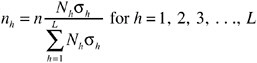
Equation 5.3 is only valid if samples are allocated in accordance with equation 5.2.

In contrast, if random sampling is performed without stratification, the required number of samples needed is: 5

where σ 2 is the population variance of samples taken from individual water use sites.

EXAMPLE: DEVELOPMENT OF A SAMPLING PLAN FOR ARKANSAS

The purpose of this example is to illustrate how a sampling approach can be used to estimate total annual withdrawals of water in the state of Arkansas. The example utilizes the existing inventory of point withdrawals within the state, which in 1997 contained 44,670 individual withdrawal points.

The 1997 Database

The 1997 database contains monthly and annual values for 44,670 groundwater and surface water withdrawal points. The information used in the analysis below includes county name, annual withdrawal, source designation, category of use, and pipe diameter. Table 5.1 contains the summary statistics for the 1997 data.

Irrigation withdrawals accounted for nearly 71 percent of the total offstream withdrawals and 92 percent of the total withdrawal points in 1997. A single withdrawal point for nuclear power accounted for nearly 12 percent of the withdrawn volume of water.

Sampling Approach

The data in Table 5.1 were obtained by using a census approach. Although state law mandates the inventory, the inventory entails a cost borne by individual water users and the state government. For all practical purposes, the 1997 data can be taken to represent the entire population of individual withdrawal points in Arkansas, providing us with accurate knowledge of population variances needed to develop a sampling plan. In usual practice, the population standard deviations would be unknown and would be estimated with sample standard deviations or historical population standard deviations.

TABLE 5.1 Database of Point Withdrawals in Arkansas, 1997

The sample size would be 35,560 withdrawal points or almost 80 percent of the population. When the population variance and the number of users are large (the typical case in water use estimation), the standard error for random sampling and the number of samples required are also very large.

However, the error can be reduced by dividing the population into distinct strata (with smaller strata variances). If optimal stratified sampling is employed, using the use categories in Table 5.1 as the strata, the total number of samples n needed to estimate water use with the same standard error is determined as follows:

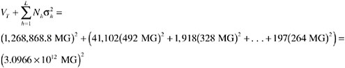
and from Equation 5.3,

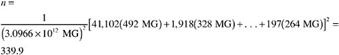
Thus, stratification has the potential to substantially improve sampling efficiency. Stratified random sampling reduces the number of samples needed by grouping water use quantities likely to be similar. In this case study, for example, large uses by power plants are separated from smaller irrigation uses, removing some of the sampling variance or randomness.

Allocating the samples according to Equation 5.2 results in the required numbers of samples within each category, as shown in the column in Table 5.2 for corrected number of samples. In two categories (hydropower and nuclear power), the calculated number of samples required exceeds the population size. This impossibility is corrected for such cases by requiring that all users be sampled. Adding an additional requirement that each category have a minimum of two samples results in the corrected values for n h in Table 5.2 .

TABLE 5.2 Number of Required Samples, by Category, to Achieve Approximately 10% Standard Error in the Water Use Estimate

Equation 5.1 allows calculation of the standard error for any sample allocation. Using this equation for the corrected n h shows that the standard error in the estimate of total use is 1,592,912 MG, or about 12.6 percent error. If this value is unacceptable, additional samples could be taken from the 10 categories containing unsampled users. Solving iteratively for the samples required to result in a standard error of 10 percent, the final numbers of required samples ( Table 5.2 ) is obtained. Thus, to achieve 10 percent standard error, the stratified random sampling approach requires 471 samples, less than 1.1 percent of the population. Within each category, random sampling is used to estimate water withdrawals.

The last column of Table 5.2 shows the standard error by category, as well as the standard error for all sectors combined. Obviously, in the two categories where all users would be sampled, the error is zero (except for unknown measurement errors). Note, however, in all other categories, the standard errors are greater than 10 percent. In some applications, sample planning may also include objectives on allowable errors for individual categories, or allowable errors for total withdrawals by county or region. If so, additional sampling would be required to meet these objectives.

SUBSTRATA DELINEATION

With the stratified random sampling approach, withdrawal measurements are made only on a subset of the population within a category/stratum. The effectiveness of the stratified random sampling approach depends on the variances of the populations within the strata. Where variances within strata are high, it may be useful to divide a stratum into two or more substrata. The equations described early in this chapter could be easily modified to address the situation where boundaries between substrata are obvious and chosen before sampling begins. In other cases, the decision about subdividing a stratum may seem arbitrary, e.g., dividing a range of users into two subcategories of major and minor users. It may be efficient in such a case to sample a smaller proportion of the minor users, particularly when the variability associated with minor users is low. This may occur, for example, when there are large numbers of users with zero withdrawal (see Table 5.1 ).

Example: Determination of Substrata Boundaries and Assessment of Errors

The main purpose of this example is to examine the precision of estimating stratum water withdrawals with an alternative sampling approach. This approach combines statistical sampling of minor withdrawal points with a census (i.e., a

complete enumeration) of major withdrawal points. It is designed to overcome the problems presented by the very heterogeneous population from which the sample is taken. In contrast to a standard sampling problem in which the sizes of the strata are predefined, this example approach simultaneously selects the sample size and the boundary between the two strata. By using an electronic spreadsheet, it is possible to calculate the population statistics for each stratum while moving the stratum boundary from the largest withdrawal points to the smallest. Points in the top stratum are individually measured (i.e., through a census), and a random sample is taken from all the remaining points in the population. If we assume a target standard error of 10 percent of the total withdrawal for groundwater and for surface water, Equation 5.4 can be used to calculate the required sample size for the bottom stratum.

The approach is applied to a single water use category: the population of Arkansas’ 1997 irrigation withdrawals. The 1997 data for Arkansas reported irrigation withdrawal volumes for 41,102 points, of which 5,417 show no water withdrawal in 1997. Table 5.3 summarizes the statistics for the subpopulations of groundwater and surface water withdrawals for irrigation.

Figure 5.1 shows the total sample size (i.e., all points in the top stratum plus sampled points in the bottom stratum) needed to achieve the target standard error as a function of top stratum size for Arkansas’ groundwater and surface water irrigation withdrawals. Note the minimum total sample size required for the groundwater subcategory is less than that for surface water subcategory, even though there are over seven times as many groundwater withdrawal points. This occurs because the relative variability is much lower for the groundwater subcategory.

Still, the delineation of a substratum boundary is very effective in reducing the sampling required for surface water. To estimate the total annual surface withdrawal for irrigation with a 10 percent standard error using random sam-

TABLE 5.3 Population Characteristics for Irrigation Withdrawals, Arkansas, 1997

FIGURE 5.1 Optimum sample size for the sampling of groundwater and surface water withdrawals for irrigation using substrata boundaries, Arkansas, 1997.

pling, the required number of samples is 1,789. Using the substratum boundary, the minimum total sample size is 163 ( Figure 5.1 ); the 60 withdrawal points with the largest annual quantities should all be measured (approximately 1.2 percent of all surface withdrawal points for irrigation), and a random sample of 103 withdrawal points (or approximately 2 percent of all points) should be selected from the remaining 4,989 withdrawal points. In contrast, the use of a substratum boundary does not significantly reduce the sampling required for groundwater. Using random sampling, the required number of samples is 110. Using the substratum boundary, the minimum total sample size is 110; the single largest withdrawal points should be measured, and a random sample of 109 points (approximately 0.3 percent) should be selected from the remaining 36,052 groundwater withdrawal points. Hence, with groundwater withdrawals for irrigation, which account for over 80 percent of all withdrawal points in the state database, random sampling is sufficient for statewide water use estimation.

Overall, the division of irrigation withdrawals into two subcategories and the use of substrata boundaries (at least for surface water) greatly improve on random sampling within the irrigation category. As shown in Table 5.2 , the use of 330 random samples as part of a statewide sampling plan results in a standard error of 16 percent for the irrigation category. Using the minimum sampling indicated above, a total of 273 samples is required, and with a standard error of about 4.4 percent for the total irrigation withdrawal (using Equation 5.1). Still, it is worth noting that there are some practical problems associated with implementing such a plan. For instance, identifying the largest users could be difficult in the absence of census data. This and other issues would need to be considered as part of the sample planning process.

APPLICATION TO STATES THAT LACK WATER USE DATA

The example analysis used known statistics for 1997 water use in Arkansas to develop an optimal sampling plan that could be used in subsequent years. This example demonstrates the substantial, optimal benefit of stratified random sampling. However, random sampling is most needed for states or programs that currently lack data on water use. In these cases, USGS researchers would not have the information needed to develop an optimal sampling plan. However, stratified random sampling can still be employed as long as it is possible to estimate the number of users in a set of use categories. This is true even in the absence of prior knowledge of the site-specific statistics. The sampling plan developed for this situation would likely be nonoptimal, but stratified random sampling does not have to be optimal to be useful. Using Equation 5.1, it is possible to estimate error variance and standard error for water use estimated from any stratified sampling plan. Water use estimates developed from nonoptimal sampling plans will be expected to have larger standard errors than estimates developed from optimal sampling plans with the same number of total samples.

increase the standard error of the water use estimate. This situation will likely improve as time passes. The statistical data collected during the first complete stratified sampling effort would be used to design an improved sampling plan for future use.

A second possibility for developing a sampling plan in the absence of prior statistics is to use category variances available from state programs with substantive data collection efforts in the optimal sampling plan Equations 5.2 and 5.3 with the target state’s category numbers. This will work best when similarities in the categorical water use between the two states are expected. Again, discrepancies between variances in the target state and the data-rich state will render the plan less than optimal, but will not impair the ability to assign an estimated error to the water use estimate.

A third possibility exists where the state has the legal authority to register or permit water withdrawals. Permitted withdrawals could be used as an approximation of actual withdrawals for the purpose of sampling plan design.

This discussion has described only a few ideas for setting up a sampling plan for the first survey when a good water use database is not available. More work is needed to expand this list and evaluate the utility of each option.

The sampling plan would also require information on the number of water users in each category. One approach would be to do a census of the water users. However, this approach might be prohibitive in most states. Alternate methods for estimating the number of water users need to be explored. The Census of Agriculture, the Population Census, manufacturing surveys, and other data sources may provide information necessary for water use population estimation (see Chapter 4 ). The USGS should also consider consulting with and using the services of experts in other federal or state agencies for help in estimating the number of water users within a state.

ISSUES FOR FURTHER RESEARCH

This is a preliminary study of data from a single state. Comparative studies of data from a number of states with differing degrees of data quality are needed to solidify the understanding of how stratified random sampling can best be applied to water use. Some of the questions that remain to be resolved are the following:

Most states have a trigger level for reporting water use, so the population of sites sampled is censored to omit the smallest users. How can stratified random sampling be used to estimate total water use from a sample censored in this manner?

A region may have a particular water use category such as irrigation, for which the total number of water withdrawal points is not known precisely and can

only be estimated. How does uncertainty in the size of the total population affect the error of estimate of total water use in the region?

What is reported on most water use surveys as the amount withdrawn or used is not a measurement but is itself an estimate by the water user. Can a measure of these site-specific estimation errors be obtained and incorporated within the error estimates for the water use strata so as to adjust the number of users sampled to allow for the estimate of the error inherent in sampling each user?

The 50 states, the District of Columbia, and Puerto Rico can be thought of as a collection of 52 sampling units, which each have particular characteristics. An attempt has been made in Chapter 2 to classify these sampling units for data quality. How can the data be examined state by state to more rigorously quantify data quality as a function of characteristics such as the type of laws pertaining to water use data collection?

In many states, the samples of water use sites, often obtained by voluntary submission of water use reports, are incomplete. Can incomplete samples of this kind be used in a stratified random sampling framework to arrive at reasonable estimates of the total water use and its standard error?

The examples presented in this chapter are all for annual withdrawals in Arkansas. Does the variability of monthly water use differ sufficiently from that of annual water use to require a different sampling plan?

Measurement errors for withdrawals were ignored in the Arkansas example. Although stratified sampling reduces the sampling requirements, it still requires quality data for water use estimation. Are modifications needed to the statistical approaches to deal with measurement uncertainty, which might vary from state to state?

The USGS has a strong group of water statisticians who have experience in examining the above issues in other contexts, such as analysis of floods, streamflow, and water quality (Helsel and Hirsch, 1992). The statistical studies recommended here are certainly within their range of competence.

CONCLUSIONS AND RECOMMENDATIONS

This chapter has described some of the potential benefits of using random sampling to estimate water use. Benefits may include reduced sampling and associated costs (compared to performing a full census), simple approaches to assessing the quality of water use estimates, as well as the ability to design a sampling plan to meet particular data-quality needs.

One important benefit of random sampling is a potential reduction in data collection efforts. By incorporating variance reduction techniques, particularly optimal stratified sampling, quality water use estimates may be obtained by sam-

pling less than 5 percent to 10 percent of users. An example analysis for Arkansas showed that only approximately 1 percent of users needed to be sampled for estimating state-level water use, with a standard error of 10 percent. A greater percentage of users would need to be sampled to achieve the same standard error for regional or county-level estimates or for estimates for individual water use categories.

Random sampling facilitates the use of statistical approaches to calculate and report the quality of water use estimates. For example, in this chapter’s analysis, standard error in water use estimates was chosen as the measure of quality. Other measures, such as confidence intervals, could also be used to describe quality.

Another advantage of random sampling is that it allows water use program staff to readily design a sampling program to meet particular data-quality needs. In the study performed earlier in this chapter, the total number of samples and the allocation of samples among strata were chosen to meet an allowable standard error. In practice, quality targets could be based on the intended uses for the data, ensuring that sampling efforts and staff resources are directed where they are most needed. Furthermore, sampling programs need not be fixed; dynamic sampling could also be beneficial. For example, if a preliminary analysis of sample data shows that variability in a particular use category is substantially higher than expected, it may make sense to update the number and allocation of samples and perform additional sampling.

Many variations on the random sampling approach are possible. The case study demonstrated the use of a hybrid approach to random sampling within a single category or stratum—samples were drawn randomly for “minor” users in the category, and a census approach was used for “major” users. The study showed that for surface water irrigation withdrawals in Arkansas, the hybrid approach required far fewer surface water samples than with random sampling. However, for groundwater irrigation withdrawals, where the relative variability of withdrawals is much lower than for surface water, the hybrid approach offers no advantage over random sampling. Further guidance is needed to help USGS districts select appropriate statistical sampling techniques for water use estimation in individual states.

The quality of results from the random sampling approach is limited by some of the same issues that affect the census approach. Although full surveys are not required of every use category, it is still critically important to have an accurate count of the total number of users. In addition, when stratified sampling is used, all users must be accurately distributed into categories. Maintaining accurate user counts may require a substantial amount of effort. In addition, whether the census approach or random sampling is used, procedures must be established to manage the response rate (e.g., follow-up for surveys not returned). Depending upon the situation, these efforts could be substantial. As a result, further study is needed to determine whether substantial cost reductions could be achieved through stratified random sampling in actual practice. The examples in this

chapter certainly support the possibility of reduced costs and justify an additional investigation.

A disadvantage of reducing the proportion of users sampled (by using random sampling rather than the census approach) is the possibility of increased uncertainty in water use estimates. Thus, it is important to ensure that sampled data are accurate and representative. However, as a result of diminishing returns (each additional sample progressively provides less information as the sample size increases), stratified random sampling has the potential for greatly reducing the data collection workload with small, acceptable increases in uncertainty. This beneficial outcome can be obtained by explicitly balancing costs and accuracy. Reducing the quantity of data collected may even allow increased attention to quality for the fewer data collected.

The committee recommends that the USGS develop statistical sampling approaches for water use estimation as part of the National Water-Use Information Program. Site-specific water use data from various states may be useful in developing and evaluating sampling approaches. The National Handbook of Recommended Methods for Water Data Acquisition (USGS, 2000) and the USGS’s internal guides for preparing water use estimates should be updated with a manual of procedures for statistical sampling of water use and determination of total water use estimates and their errors.

Across the United States, the practices for collecting water use data vary significantly from state to state and vary also from one water use category to another, in response to the laws regulating water use and interest in water use data as an input for water management. However, many rich bodies of water use data exist at the state level, and an outstanding opportunity exists for assembling and statistically analyzing these data at the national level. This would lead to better techniques for water use estimation and to a greater capacity to link water use with its impact on water resources.

This report is a product of the Committee on Water Resources Research, which provides consensus advice to the Water Resources Division (WRD) of the USGS on scientific, research, and programmatic issues. The committee works under the auspices of the Water Science and Technology Board of the National Research Council (NRC). The committee considers a variety of topics that are important scientifically and programmatically to the USGS and the nation and issues reports when appropriate. This report concerns the National Water-Use Information Program (NWUIP).

READ FREE ONLINE

Welcome to OpenBook!

You're looking at OpenBook, NAP.edu's online reading room since 1999. Based on feedback from you, our users, we've made some improvements that make it easier than ever to read thousands of publications on our website.

Do you want to take a quick tour of the OpenBook's features?

Show this book's table of contents , where you can jump to any chapter by name.

...or use these buttons to go back to the previous chapter or skip to the next one.

Jump up to the previous page or down to the next one. Also, you can type in a page number and press Enter to go directly to that page in the book.

Switch between the Original Pages , where you can read the report as it appeared in print, and Text Pages for the web version, where you can highlight and search the text.

To search the entire text of this book, type in your search term here and press Enter .

Share a link to this book page on your preferred social network or via email.

View our suggested citation for this chapter.

Ready to take your reading offline? Click here to buy this book in print or download it as a free PDF, if available.

Get Email Updates

Do you enjoy reading reports from the Academies online for free ? Sign up for email notifications and we'll let you know about new publications in your areas of interest when they're released.