assignment for hybridization

Home / How To Determine Hybridization: A Shortcut

Bonding, Structure, and Resonance

By James Ashenhurst

• How To Determine Hybridization: A Shortcut

Last updated: December 28th, 2022 |

A Shortcut For Determining The Hybridization Of An Atom In A Molecule

Here’s a shortcut for how to determine the hybridization of an atom in a molecule that will work in at least 95% of the cases you see in Org 1. 

For a given atom:

• Count the number of atoms connected to it (atoms – not bonds!)
• Count the number of lone pairs attached to it.
• Add these two numbers together.
• If it’s 4 , your atom is sp 3 .
• If it’s 3 , your atom is sp 2 .
• If it’s 2 , your atom is sp. 

(If it’s 1, it’s probably hydrogen!)

The main exception is atoms with lone pairs that are adjacent to pi bonds, which we’ll discuss in detail below.

Table of Contents

• Some Simple Worked Examples Of The Hybridization Shortcut
• How To Determine Hybridization Of An Atom: Two Exercises
• Are There Any Exceptions?
• Exception #1: Lone Pairs Adjacent To Pi-bonds
• Lone Pairs In P-Orbitals (Versus Hybrid Orbitals) Have Better Orbital Overlap With Adjacent Pi Systems
• Exception #2. Geometric Constraints
• “Geometry Determines Hybridization, Not The Other Way Around”

1. Some Simple Worked Examples Of The Hybridization Shortcut

sp 3 hybridization : sum of attached atoms + lone pairs = 4

sp 2 hybridization : sum of attached atoms + lone pairs = 3

sp hybridization : sum of attached atoms + lone pairs = 2

Where it can start to get slightly tricky is in dealing with line diagrams containing implicit (“hidden”) hydrogens and lone pairs.

Chemists like time-saving shortcuts just as much as anybody else, and learning to quickly interpret line diagrams is as fundamental to organic chemistry as learning the alphabet is to written English.

• Just because lone pairs aren’t drawn in on oxygen, nitrogen, and fluorine doesn’t mean they’re not there.
• Assume a full octet for C, N, O, and F with the following  one exception: a positive charge on carbon indicates that there are only six electrons around it. [ Nitrogen and oxygen bearing a formal charge of +1 still have full octets].

[ Advanced: Note 1 covers how to determine the hybridization of atoms in some weird cases like free radicals, carbenes and nitrenes ]

2. How To Determine Hybridization Of An Atom: Two Exercises

Here’s an exercise. Try picking out the hybridization of the atoms in this highly poisonous molecule made by the frog in funky looking pyjamas, below right.

[Don’t worry if the molecule looks a little crazy: just focus on the  individual atoms  that the arrows point to (A, B, C, D, E). A and B especially.  If you haven’t mastered line diagrams yet ( and “hidden” hydrogens ) maybe get some more practice and come back to this later.]

Here are some more examples.

More practice quizzes for hybridization can be found here (MOC Membership unlocks them all)

3. Are There Any Exceptions? 

Sure.  Although as with many things, explaining the shortcut takes about 2 minutes, while explaining the exceptions takes about 10 times longer.

Helpfully, these exceptions fall into two main categories. It should be noted that by the time your course explains why these examples are exceptions, it will likely have moved far beyond hybridization.

Bottom line: these probably won’t be found on your first midterm.

4. Exception #1: Lone Pairs Adjacent To Pi-bonds 

The main exception is for atoms bearing lone pairs that are adjacent to pi bonds.

Quick shortcut: Lone pairs adjacent to pi-bonds (and pi-systems) tend to be in unhybridized p orbitals, rather than in hybridized sp n  orbitals.

This is most common for  nitrogen  and  oxygen .

In the cases below, a nitrogen or oxygen that we might expect to be sp 3 hybridized is actually sp 2 hybridized (trigonal planar).

Why? The quick answer is that lowering of energy from  conjugation of the p-orbital with the adjacent pi-bond more than compensates for the rise in energy due to greater electron-pair repulsion for sp 2 versus sp 3

[see this post: “ Conjugation and Resonance “]

What’s the long answer?

5. Lone Pairs In P-Orbitals (Versus Hybrid Orbitals) Have Better Orbital Overlap With Adjacent Pi Systems

Let’s think back to why atoms hybridize in the first place: minimization of electron-pair repulsion.

For a primary amine like methylamine, adoption of a tetrahedral (sp 3 ) geometry by nitrogen versus a trigonal planar (sp 2 ) geometry is worth about 5 kcal/mol [roughly 20 kJ/mol].

That might not sound like a lot, but for two species in equilibrium, a difference of 5 kcal/mol in energy represents a ratio of about 4400:1 ] . [How do we know this? See this (advanced) Note 2 on nitrogen inversion] 

What if there was some compensating effect whereby a lone pair unhybridized p-orbital was actually more stable than if it was in a hybridized orbital?

This turns out to be the case in many situations where the lone pair is adjacent to a pi bond!  The most common and important example is that of amides , which constitute the linkages between amino acids. The nitrogen in amides is planar (sp 2 ), not trigonal pyramidal (sp 3 ), as proven by x-ray crystallography.

The difference in energy varies widely, but a typical value is about 10 kcal/mol favouring the trigonal planar geometry.  [We know this because many amides have a measurable barrier to rotation a topic we also talked about in the Conjugation and Resonance post]

Why is trigonal planar geometry favoured here? Better orbital overlap of the p orbital with the pi bond vs. the (hybridized) sp 3 orbital .

You can think of this as leading to a stronger “partial” C–N bond. Two important consequences of this interaction are  restricted rotation in amides, as well as the fact that acid reacts with amides on the oxygen, not the nitrogen lone pair (!)

The oxygen in esters and enols is also also sp 2 hybridized, as is the nitrogen in enamines and countless other examples.

As you will likely see in Org 2, some of the most dramatic cases are those where the “de-hybridized” lone pair participates in an aromatic system . Here, the energetic compensation for a change in hybridization from sp 3 to sp 2 can be very great indeed – more than 20 kcal/mol in some cases.

For this reason, the most basic site of pyrrole is not the nitrogen lone pair, but on the carbon (C-2) (!).

6. Exception #2. Geometric Constraints

Another example where the actual hybridization differs from what we might expect from the shortcut is in cases with geometric constraints. For instance in the phenyl cation below, the indicated carbon is attached two two atoms and zero lone pairs.

What’s the hybridization?

From our shortcut, we might expect the hybridization to be sp .

In fact, the geometry around the atom is much closer to sp 2 . That’s because the angle strain adopting the linear (sp) geometry would lead to far too much angle strain to be a stable molecule.

7. “Geometry Determines Hybridization, Not The Other Way Around”

A quote passed on to me from Matt seems appropriate:

“Geometry determines hybridization, not the other way around”

Well, that’s probably more than you wanted to know about how to determine the hybridization of atoms.

Suffice to say, any post from this site that contains shortcut in the title is a sure fire-bet to have over 1000 words and >10 figures.

Thanks to Matt Pierce of  Organic Chemistry Solutions   for important contributions to this post.  Ask Matt about scheduling an online tutoring session  here .

Related Articles

• Hidden Hydrogens, Hidden Lone Pairs, Hidden Counterions
• Hybrid Orbitals and Hybridization
• How Do We Know Methane (CH4) Is Tetrahedral?
• Orbital Hybridization And Bond Strengths
• Conjugation And Resonance In Organic Chemistry
• Bond Hybridization Practice (MOC Membership)

Note 1. Some weird cases.

Sometimes you might be asked to determine the hybridization of  free radicals and of  carbenes  (or nitrenes)

Although you’re unlikely to encounter these, let’s still have a look.

• Free radicals exist in a shallow pyramidal  geometry, not purely sp 2 or sp 3 .
• However, if they are  adjacent to a pi system (e.g. a C-C double or triple bond) then the shallow pyramid will  re-hybridize to give it an sp 2 geometry, which allows for full resonance delocalization of the free radical.
• Carbenes and  nitrenes would give us sp 2 geometry by the hybridization shortcut. However their actual structures can vary depending on whether or not the electron pair exists in a single orbital (a  singlet carbene) or is divided into two singly-filled orbitals (a  triplet carbene). That’s really beyond the scope of introductory organic chemistry.

What about higher block elements like sulfur and phosphorus?

Third row elements like phosphorus and sulfur can exceed an octet of electrons by incorporating d-orbitals in the hybrid.  This is more in the realm of inorganic chemistry so I don’t really want to discuss it. Here’s an example for the hybridization of SF 4 from elsewhere .  (sp 3 d orbitals).

Note 2 : For the 5 kcal/mol figure, see here . [Tetrahedron Lett, 1971, 37 , 3437]. (Kurt Mislow, RIP . )

An amine connected to three different substituents (R 1 R 2 and R 3 ) should be chiral, since it has in total 4 different substituents (including the lone pair). However, all early attempts to prepare enantiomerically pure amines met with failure. It was later found that amines undergo inversion at room temperature, like an umbrella being forced inside-out by a strong wind.

In the transition state for inversion the nitrogen is trigonal planar. One can thus calculate the difference in energy between the sp 3 and sp 2 geometries by measuring the activation barrier for this process (see ref ).

Note 3 :A fun counter-example might be Coelenterazine  .

One would not expect both nitrogen atoms to be sp 2 hybridized, because that would lead to a cyclic, flat, conjugated system with 8 pi electrons : in other words, antiaromatic. I can’t find a crystal structure of the core molecule to confirm (but would welcome any additional information!)

NOTE – (added afterwards) If you draw the resonance form where the nitrogen lone pair forms a pi bond with the carbonyl carbon, then the ring system has 10 electrons and would therefore be “aromatic”.

• Barrier to pyramidal inversion of nitrogen in dibenzylmethylamine Michael J. S. Dewar and W. Brian Jennings Journal of the American Chemical Society   1971   93 (2), 401-403 DOI: 10.1021/ja00731a016

Pyramidal inversion barriers: the significance of ground state geometry Joseph Stackhouse, Raymond D.Baechler, Kurt Mislow Tetrahedron Letters  Volume 12, Issue 37,  1971 , Pages 3437-3440 DOI: doi.org/10.1016/S0040-4039(01)97199-0

00 General Chemistry Review

• Lewis Structures
• Ionic and Covalent Bonding
• Chemical Kinetics
• Chemical Equilibria
• Valence Electrons of the First Row Elements
• How Concepts Build Up In Org 1 ("The Pyramid")

01 Bonding, Structure, and Resonance

• Sigma bonds come in six varieties: Pi bonds come in one
• A Key Skill: How to Calculate Formal Charge
• The Four Intermolecular Forces and How They Affect Boiling Points
• 3 Trends That Affect Boiling Points
• How To Use Electronegativity To Determine Electron Density (and why NOT to trust formal charge)
• Introduction to Resonance
• How To Use Curved Arrows To Interchange Resonance Forms
• Evaluating Resonance Forms (1) - The Rule of Least Charges
• How To Find The Best Resonance Structure By Applying Electronegativity
• Evaluating Resonance Structures With Negative Charges
• Evaluating Resonance Structures With Positive Charge
• Exploring Resonance: Pi-Donation
• Exploring Resonance: Pi-acceptors
• In Summary: Evaluating Resonance Structures
• Drawing Resonance Structures: 3 Common Mistakes To Avoid
• How to apply electronegativity and resonance to understand reactivity
• Bond Hybridization Practice
• Structure and Bonding Practice Quizzes
• Resonance Structures Practice

02 Acid Base Reactions

• Introduction to Acid-Base Reactions
• Acid Base Reactions In Organic Chemistry
• The Stronger The Acid, The Weaker The Conjugate Base
• Walkthrough of Acid-Base Reactions (3) - Acidity Trends
• Five Key Factors That Influence Acidity
• Acid-Base Reactions: Introducing Ka and pKa
• How to Use a pKa Table
• The pKa Table Is Your Friend
• A Handy Rule of Thumb for Acid-Base Reactions
• Acid Base Reactions Are Fast
• pKa Values Span 60 Orders Of Magnitude
• How Protonation and Deprotonation Affect Reactivity
• Acid Base Practice Problems

03 Alkanes and Nomenclature

• Meet the (Most Important) Functional Groups
• Condensed Formulas: Deciphering What the Brackets Mean
• Don't Be Futyl, Learn The Butyls
• Primary, Secondary, Tertiary, Quaternary In Organic Chemistry
• Branching, and Its Affect On Melting and Boiling Points
• The Many, Many Ways of Drawing Butane
• Wedge And Dash Convention For Tetrahedral Carbon
• Common Mistakes in Organic Chemistry: Pentavalent Carbon
• Table of Functional Group Priorities for Nomenclature
• Summary Sheet - Alkane Nomenclature
• Organic Chemistry IUPAC Nomenclature Demystified With A Simple Puzzle Piece Approach
• Boiling Point Quizzes
• Organic Chemistry Nomenclature Quizzes

04 Conformations and Cycloalkanes

• Staggered vs Eclipsed Conformations of Ethane
• Conformational Isomers of Propane
• Newman Projection of Butane (and Gauche Conformation)
• Introduction to Cycloalkanes (1)
• Geometric Isomers In Small Rings: Cis And Trans Cycloalkanes
• Calculation of Ring Strain In Cycloalkanes
• Cycloalkanes - Ring Strain In Cyclopropane And Cyclobutane
• Cyclohexane Conformations
• Cyclohexane Chair Conformation: An Aerial Tour
• How To Draw The Cyclohexane Chair Conformation
• The Cyclohexane Chair Flip
• The Cyclohexane Chair Flip - Energy Diagram
• Substituted Cyclohexanes - Axial vs Equatorial
• Ranking The Bulkiness Of Substituents On Cyclohexanes: "A-Values"
• Cyclohexane Chair Conformation Stability: Which One Is Lower Energy?
• Fused Rings - Cis-Decalin and Trans-Decalin
• Naming Bicyclic Compounds - Fused, Bridged, and Spiro
• Bredt's Rule (And Summary of Cycloalkanes)
• Newman Projection Practice
• Cycloalkanes Practice Problems

05 A Primer On Organic Reactions

• The Most Important Question To Ask When Learning a New Reaction
• Learning New Reactions: How Do The Electrons Move?
• The Third Most Important Question to Ask When Learning A New Reaction
• 7 Factors that stabilize negative charge in organic chemistry
• 7 Factors That Stabilize Positive Charge in Organic Chemistry
• Nucleophiles and Electrophiles
• Curved Arrows (for reactions)
• Curved Arrows (2): Initial Tails and Final Heads
• Nucleophilicity vs. Basicity
• The Three Classes of Nucleophiles
• What Makes A Good Nucleophile?
• What makes a good leaving group?
• 3 Factors That Stabilize Carbocations
• Equilibrium and Energy Relationships
• What's a Transition State?
• Hammond's Postulate
• Learning Organic Chemistry Reactions: A Checklist (PDF)
• Introduction to Free Radical Substitution Reactions
• Introduction to Oxidative Cleavage Reactions

06 Free Radical Reactions

• Bond Dissociation Energies = Homolytic Cleavage
• Free Radical Reactions
• 3 Factors That Stabilize Free Radicals
• What Factors Destabilize Free Radicals?
• Bond Strengths And Radical Stability
• Free Radical Initiation: Why Is "Light" Or "Heat" Required?
• Initiation, Propagation, Termination
• Monochlorination Products Of Propane, Pentane, And Other Alkanes
• Selectivity In Free Radical Reactions
• Selectivity in Free Radical Reactions: Bromination vs. Chlorination
• Halogenation At Tiffany's
• Allylic Bromination
• Bonus Topic: Allylic Rearrangements
• In Summary: Free Radicals
• Synthesis (2) - Reactions of Alkanes
• Free Radicals Practice Quizzes

07 Stereochemistry and Chirality

• Types of Isomers: Constitutional Isomers, Stereoisomers, Enantiomers, and Diastereomers
• How To Draw The Enantiomer Of A Chiral Molecule
• How To Draw A Bond Rotation
• Introduction to Assigning (R) and (S): The Cahn-Ingold-Prelog Rules
• Assigning Cahn-Ingold-Prelog (CIP) Priorities (2) - The Method of Dots
• Enantiomers vs Diastereomers vs The Same? Two Methods For Solving Problems
• Assigning R/S To Newman Projections (And Converting Newman To Line Diagrams)
• How To Determine R and S Configurations On A Fischer Projection
• The Meso Trap
• Optical Rotation, Optical Activity, and Specific Rotation
• Optical Purity and Enantiomeric Excess
• What's a Racemic Mixture?
• Chiral Allenes And Chiral Axes
• Stereochemistry Practice Problems and Quizzes

08 Substitution Reactions

• Introduction to Nucleophilic Substitution Reactions
• Walkthrough of Substitution Reactions (1) - Introduction
• Two Types of Nucleophilic Substitution Reactions
• The SN2 Mechanism
• Why the SN2 Reaction Is Powerful
• The SN1 Mechanism
• The Conjugate Acid Is A Better Leaving Group
• Comparing the SN1 and SN2 Reactions
• Polar Protic? Polar Aprotic? Nonpolar? All About Solvents
• Steric Hindrance is Like a Fat Goalie
• Common Blind Spot: Intramolecular Reactions
• The Conjugate Base is Always a Stronger Nucleophile
• Substitution Practice - SN1
• Substitution Practice - SN2

09 Elimination Reactions

• Elimination Reactions (1): Introduction And The Key Pattern
• Elimination Reactions (2): The Zaitsev Rule
• Elimination Reactions Are Favored By Heat
• Two Elimination Reaction Patterns
• The E1 Reaction
• The E2 Mechanism
• E1 vs E2: Comparing the E1 and E2 Reactions
• Antiperiplanar Relationships: The E2 Reaction and Cyclohexane Rings
• Bulky Bases in Elimination Reactions
• Comparing the E1 vs SN1 Reactions
• Elimination (E1) Reactions With Rearrangements
• E1cB - Elimination (Unimolecular) Conjugate Base
• Elimination (E1) Practice Problems And Solutions
• Elimination (E2) Practice Problems and Solutions

10 Rearrangements

• Introduction to Rearrangement Reactions
• Rearrangement Reactions (1) - Hydride Shifts
• Carbocation Rearrangement Reactions (2) - Alkyl Shifts
• Pinacol Rearrangement
• The SN1, E1, and Alkene Addition Reactions All Pass Through A Carbocation Intermediate

11 SN1/SN2/E1/E2 Decision

• Identifying Where Substitution and Elimination Reactions Happen
• Deciding SN1/SN2/E1/E2 (1) - The Substrate
• Deciding SN1/SN2/E1/E2 (2) - The Nucleophile/Base
• SN1 vs E1 and SN2 vs E2 : The Temperature
• Deciding SN1/SN2/E1/E2 - The Solvent
• Wrapup: The Key Factors For Determining SN1/SN2/E1/E2
• Alkyl Halide Reaction Map And Summary
• SN1 SN2 E1 E2 Practice Problems

12 Alkene Reactions

• E and Z Notation For Alkenes (+ Cis/Trans)
• Alkene Stability
• Alkene Addition Reactions: "Regioselectivity" and "Stereoselectivity" (Syn/Anti)
• Stereoselective and Stereospecific Reactions
• Hydrohalogenation of Alkenes and Markovnikov's Rule
• Hydration of Alkenes With Aqueous Acid
• Rearrangements in Alkene Addition Reactions
• Halogenation of Alkenes and Halohydrin Formation
• Oxymercuration Demercuration of Alkenes
• Hydroboration Oxidation of Alkenes
• m-CPBA (meta-chloroperoxybenzoic acid)
• OsO4 (Osmium Tetroxide) for Dihydroxylation of Alkenes
• Palladium on Carbon (Pd/C) for Catalytic Hydrogenation of Alkenes
• Cyclopropanation of Alkenes
• A Fourth Alkene Addition Pattern - Free Radical Addition
• Alkene Reactions: Ozonolysis
• Summary: Three Key Families Of Alkene Reaction Mechanisms
• Synthesis (4) - Alkene Reaction Map, Including Alkyl Halide Reactions
• Alkene Reactions Practice Problems

13 Alkyne Reactions

• Acetylides from Alkynes, And Substitution Reactions of Acetylides
• Partial Reduction of Alkynes With Lindlar's Catalyst
• Partial Reduction of Alkynes With Na/NH3 To Obtain Trans Alkenes
• Alkyne Hydroboration With "R2BH"
• Hydration and Oxymercuration of Alkynes
• Hydrohalogenation of Alkynes
• Alkyne Halogenation: Bromination, Chlorination, and Iodination of Alkynes
• Alkyne Reactions - The "Concerted" Pathway
• Alkenes To Alkynes Via Halogenation And Elimination Reactions
• Alkynes Are A Blank Canvas
• Synthesis (5) - Reactions of Alkynes
• Alkyne Reactions Practice Problems With Answers

14 Alcohols, Epoxides and Ethers

• Alcohols - Nomenclature and Properties
• Alcohols Can Act As Acids Or Bases (And Why It Matters)
• Alcohols - Acidity and Basicity
• The Williamson Ether Synthesis
• Ethers From Alkenes, Tertiary Alkyl Halides and Alkoxymercuration
• Alcohols To Ethers via Acid Catalysis
• Cleavage Of Ethers With Acid
• Epoxides - The Outlier Of The Ether Family
• Opening of Epoxides With Acid
• Epoxide Ring Opening With Base
• Making Alkyl Halides From Alcohols
• Tosylates And Mesylates
• PBr3 and SOCl2
• Elimination Reactions of Alcohols
• Elimination of Alcohols To Alkenes With POCl3
• Alcohol Oxidation: "Strong" and "Weak" Oxidants
• Demystifying The Mechanisms of Alcohol Oxidations
• Protecting Groups For Alcohols
• Thiols And Thioethers
• Calculating the oxidation state of a carbon
• Oxidation and Reduction in Organic Chemistry
• Oxidation Ladders
• SOCl2 Mechanism For Alcohols To Alkyl Halides: SN2 versus SNi
• Alcohol Reactions Roadmap (PDF)
• Alcohol Reaction Practice Problems
• Epoxide Reaction Quizzes
• Oxidation and Reduction Practice Quizzes

15 Organometallics

• What's An Organometallic?
• Formation of Grignard and Organolithium Reagents
• Organometallics Are Strong Bases
• Reactions of Grignard Reagents
• Protecting Groups In Grignard Reactions
• Synthesis Problems Involving Grignard Reagents
• Grignard Reactions And Synthesis (2)
• Organocuprates (Gilman Reagents): How They're Made
• Gilman Reagents (Organocuprates): What They're Used For
• The Heck, Suzuki, and Olefin Metathesis Reactions (And Why They Don't Belong In Most Introductory Organic Chemistry Courses)
• Reaction Map: Reactions of Organometallics
• Grignard Practice Problems

16 Spectroscopy

• Degrees of Unsaturation (or IHD, Index of Hydrogen Deficiency)
• Conjugation And Color (+ How Bleach Works)
• Introduction To UV-Vis Spectroscopy
• UV-Vis Spectroscopy: Absorbance of Carbonyls
• UV-Vis Spectroscopy: Practice Questions
• Bond Vibrations, Infrared Spectroscopy, and the "Ball and Spring" Model
• Infrared Spectroscopy: A Quick Primer On Interpreting Spectra
• IR Spectroscopy: 4 Practice Problems
• 1H NMR: How Many Signals?
• Homotopic, Enantiotopic, Diastereotopic
• Diastereotopic Protons in 1H NMR Spectroscopy: Examples
• C13 NMR - How Many Signals
• Liquid Gold: Pheromones In Doe Urine
• Natural Product Isolation (1) - Extraction
• Natural Product Isolation (2) - Purification Techniques, An Overview
• Structure Determination Case Study: Deer Tarsal Gland Pheromone

17 Dienes and MO Theory

• What To Expect In Organic Chemistry 2
• Are these molecules conjugated?
• Bonding And Antibonding Pi Orbitals
• Molecular Orbitals of The Allyl Cation, Allyl Radical, and Allyl Anion
• Pi Molecular Orbitals of Butadiene
• Reactions of Dienes: 1,2 and 1,4 Addition
• Thermodynamic and Kinetic Products
• More On 1,2 and 1,4 Additions To Dienes
• s-cis and s-trans
• The Diels-Alder Reaction
• Cyclic Dienes and Dienophiles in the Diels-Alder Reaction
• Stereochemistry of the Diels-Alder Reaction
• Exo vs Endo Products In The Diels Alder: How To Tell Them Apart
• HOMO and LUMO In the Diels Alder Reaction
• Why Are Endo vs Exo Products Favored in the Diels-Alder Reaction?
• Diels-Alder Reaction: Kinetic and Thermodynamic Control
• The Retro Diels-Alder Reaction
• The Intramolecular Diels Alder Reaction
• Regiochemistry In The Diels-Alder Reaction
• The Cope and Claisen Rearrangements
• Electrocyclic Reactions
• Electrocyclic Ring Opening And Closure (2) - Six (or Eight) Pi Electrons
• Diels Alder Practice Problems
• Molecular Orbital Theory Practice

18 Aromaticity

• Introduction To Aromaticity
• Rules For Aromaticity
• Huckel's Rule: What Does 4n+2 Mean?
• Aromatic, Non-Aromatic, or Antiaromatic? Some Practice Problems
• Antiaromatic Compounds and Antiaromaticity
• The Pi Molecular Orbitals of Benzene
• The Pi Molecular Orbitals of Cyclobutadiene
• Frost Circles
• Aromaticity Practice Quizzes

19 Reactions of Aromatic Molecules

• Electrophilic Aromatic Substitution: Introduction
• Activating and Deactivating Groups In Electrophilic Aromatic Substitution
• Electrophilic Aromatic Substitution - The Mechanism
• Ortho-, Para- and Meta- Directors in Electrophilic Aromatic Substitution
• Understanding Ortho, Para, and Meta Directors
• Why are halogens ortho- para- directors?
• Disubstituted Benzenes: The Strongest Electron-Donor "Wins"
• Electrophilic Aromatic Substitutions (1) - Halogenation of Benzene
• Electrophilic Aromatic Substitutions (2) - Nitration and Sulfonation
• EAS Reactions (3) - Friedel-Crafts Acylation and Friedel-Crafts Alkylation
• Intramolecular Friedel-Crafts Reactions
• Nucleophilic Aromatic Substitution (NAS)
• Nucleophilic Aromatic Substitution (2) - The Benzyne Mechanism
• Reactions on the "Benzylic" Carbon: Bromination And Oxidation
• The Wolff-Kishner, Clemmensen, And Other Carbonyl Reductions
• More Reactions on the Aromatic Sidechain: Reduction of Nitro Groups and the Baeyer Villiger
• Aromatic Synthesis (1) - "Order Of Operations"
• Synthesis of Benzene Derivatives (2) - Polarity Reversal
• Aromatic Synthesis (3) - Sulfonyl Blocking Groups
• Birch Reduction
• Synthesis (7): Reaction Map of Benzene and Related Aromatic Compounds
• Aromatic Reactions and Synthesis Practice
• Electrophilic Aromatic Substitution Practice Problems

20 Aldehydes and Ketones

• What's The Alpha Carbon In Carbonyl Compounds?
• Nucleophilic Addition To Carbonyls
• Aldehydes and Ketones: 14 Reactions With The Same Mechanism
• Sodium Borohydride (NaBH4) Reduction of Aldehydes and Ketones
• Grignard Reagents For Addition To Aldehydes and Ketones
• Wittig Reaction
• Hydrates, Hemiacetals, and Acetals
• Imines - Properties, Formation, Reactions, and Mechanisms
• All About Enamines
• Breaking Down Carbonyl Reaction Mechanisms: Reactions of Anionic Nucleophiles (Part 2)
• Aldehydes Ketones Reaction Practice

21 Carboxylic Acid Derivatives

• Nucleophilic Acyl Substitution (With Negatively Charged Nucleophiles)
• Addition-Elimination Mechanisms With Neutral Nucleophiles (Including Acid Catalysis)
• Basic Hydrolysis of Esters - Saponification
• Transesterification
• Proton Transfer
• Fischer Esterification - Carboxylic Acid to Ester Under Acidic Conditions
• Lithium Aluminum Hydride (LiAlH4) For Reduction of Carboxylic Acid Derivatives
• LiAlH[Ot-Bu]3 For The Reduction of Acid Halides To Aldehydes
• Di-isobutyl Aluminum Hydride (DIBAL) For The Partial Reduction of Esters and Nitriles
• Amide Hydrolysis
• Thionyl Chloride (SOCl2)
• Diazomethane (CH2N2)
• Carbonyl Chemistry: Learn Six Mechanisms For the Price Of One
• Making Music With Mechanisms (PADPED)
• Carboxylic Acid Derivatives Practice Questions

22 Enols and Enolates

• Keto-Enol Tautomerism
• Enolates - Formation, Stability, and Simple Reactions
• Kinetic Versus Thermodynamic Enolates
• Aldol Addition and Condensation Reactions
• Reactions of Enols - Acid-Catalyzed Aldol, Halogenation, and Mannich Reactions
• Claisen Condensation and Dieckmann Condensation
• Decarboxylation
• The Malonic Ester and Acetoacetic Ester Synthesis
• The Michael Addition Reaction and Conjugate Addition
• The Robinson Annulation
• Haloform Reaction
• The Hell–Volhard–Zelinsky Reaction
• Enols and Enolates Practice Quizzes
• The Amide Functional Group: Properties, Synthesis, and Nomenclature
• Basicity of Amines And pKaH
• 5 Key Basicity Trends of Amines
• The Mesomeric Effect And Aromatic Amines
• Nucleophilicity of Amines
• Alkylation of Amines (Sucks!)
• Reductive Amination
• The Gabriel Synthesis
• Some Reactions of Azides
• The Hofmann Elimination
• The Hofmann and Curtius Rearrangements
• The Cope Elimination
• Protecting Groups for Amines - Carbamates
• The Strecker Synthesis of Amino Acids
• Introduction to Peptide Synthesis
• Reactions of Diazonium Salts: Sandmeyer and Related Reactions
• Amine Practice Questions

24 Carbohydrates

• D and L Notation For Sugars
• Pyranoses and Furanoses: Ring-Chain Tautomerism In Sugars
• What is Mutarotation?
• Reducing Sugars
• The Big Damn Post Of Carbohydrate-Related Chemistry Definitions
• The Haworth Projection
• Converting a Fischer Projection To A Haworth (And Vice Versa)
• Reactions of Sugars: Glycosylation and Protection
• The Ruff Degradation and Kiliani-Fischer Synthesis
• Isoelectric Points of Amino Acids (and How To Calculate Them)
• Carbohydrates Practice
• Amino Acid Quizzes

25 Fun and Miscellaneous

• A Gallery of Some Interesting Molecules From Nature
• Screw Organic Chemistry, I'm Just Going To Write About Cats
• On Cats, Part 1: Conformations and Configurations
• On Cats, Part 2: Cat Line Diagrams
• On Cats, Part 4: Enantiocats
• On Cats, Part 6: Stereocenters
• Organic Chemistry Is Shit
• The Organic Chemistry Behind "The Pill"
• Maybe they should call them, "Formal Wins" ?
• Why Do Organic Chemists Use Kilocalories?
• The Principle of Least Effort
• Organic Chemistry GIFS - Resonance Forms
• Reproducibility In Organic Chemistry
• What Holds The Nucleus Together?
• How Reactions Are Like Music
• Organic Chemistry and the New MCAT

26 Organic Chemistry Tips and Tricks

• Common Mistakes: Formal Charges Can Mislead
• Partial Charges Give Clues About Electron Flow
• Draw The Ugly Version First
• Organic Chemistry Study Tips: Learn the Trends
• The 8 Types of Arrows In Organic Chemistry, Explained
• Top 10 Skills To Master Before An Organic Chemistry 2 Final
• Common Mistakes with Carbonyls: Carboxylic Acids... Are Acids!
• Planning Organic Synthesis With "Reaction Maps"
• Alkene Addition Pattern #1: The "Carbocation Pathway"
• Alkene Addition Pattern #2: The "Three-Membered Ring" Pathway
• Alkene Addition Pattern #3: The "Concerted" Pathway
• Number Your Carbons!
• The 4 Major Classes of Reactions in Org 1
• How (and why) electrons flow
• Grossman's Rule
• Three Exam Tips
• A 3-Step Method For Thinking Through Synthesis Problems
• Putting It Together
• Putting Diels-Alder Products in Perspective
• The Ups and Downs of Cyclohexanes
• The Most Annoying Exceptions in Org 1 (Part 1)
• The Most Annoying Exceptions in Org 1 (Part 2)
• The Marriage May Be Bad, But the Divorce Still Costs Money
• 9 Nomenclature Conventions To Know
• Nucleophile attacks Electrophile

27 Case Studies of Successful O-Chem Students

• Success Stories: How Corina Got The The "Hard" Professor - And Got An A+ Anyway
• How Helena Aced Organic Chemistry
• From a "Drop" To B+ in Org 2 – How A Hard Working Student Turned It Around
• How Serge Aced Organic Chemistry
• Success Stories: How Zach Aced Organic Chemistry 1
• Success Stories: How Kari Went From C– to B+
• How Esther Bounced Back From a "C" To Get A's In Organic Chemistry 1 And 2
• How Tyrell Got The Highest Grade In Her Organic Chemistry Course
• This Is Why Students Use Flashcards
• Success Stories: How Stu Aced Organic Chemistry
• How John Pulled Up His Organic Chemistry Exam Grades
• Success Stories: How Nathan Aced Organic Chemistry (Without It Taking Over His Life)
• How Chris Aced Org 1 and Org 2
• Interview: How Jay Got an A+ In Organic Chemistry
• How to Do Well in Organic Chemistry: One Student's Advice
• "America's Top TA" Shares His Secrets For Teaching O-Chem
• "Organic Chemistry Is Like..." - A Few Metaphors
• How To Do Well In Organic Chemistry: Advice From A Tutor
• Guest post: "I went from being afraid of tests to actually looking forward to them".

Comment section

39 thoughts on “ how to determine hybridization: a shortcut ”.

i am in love with this site….. explains so clear and good….. really man i was irritated because i was not able to understand but now i understand it just because of this site….

Sir thankyou so much for your explain , i was able to get a lot of things I couldn’t understand earlier, thanks a lot ,but I have a doubt about the last note ….how did it go from antiaromatic to aromatic in coelentrazine

• Pingback: How To Determine Hybridization: A Shortcut | Straight A Mindset

Thank you for the great post, as usual.

I think there is a typo in the first section of point 5 and its picture; the geometry is trigonal pyramidal instead of tetrahedral.

very helpful thanks a lot SIR

• Pingback: Hybridization involving s, p and d-Orbitals - Overall Science

thank youuuuu!!! your discussions really helped my laboratory report in organic chemistry which is due tomorrow. can you have a discussion about the effect of pi systems? i’m looking forward to it!

may i ask for the carbon hybridization of pentane and the effects of the pi system.

Pentane, C5H12 ? Tetrahedral carbons, sp3 hybridized

Well I don’t know what to say is was really helpful to I was able to understand it thank u very much

Hi James! Firstly, thank you so much for your explanation of hybridization! Here I have a question. It says if atom with lone pair next to pi bond, rehydridization will occur so we cannot use the instruction above. So how can we determine whether an atom with lone pair is next to pi bond. Thank you!

Hi, most familiar example would be the lone pairs on the OH group of a carboxylic acid, R-CO2H. The OH oxygen is sp2 hybridized since the lone pair is on an atom adjacent to a pi bond (i.e. the C=O pi bond). Another example would be an ester, R-CO2CH3 . In this case the lone pair on the oxygen bearing the CH3 (i.e. O-CH3) is sp2 hybridized since it is adjacent to a C=O bond. Amides, R-C(O)-NH2 have sp2-hybridized nitrogens, since the lone pair on the nitrogen is adjacent to a C=O bond. The negatively charged carbon in the “allyl anion” is sp2 hybridized. Lots more examples but these are a few.

This was a great review! I hadn’t done nitrogen hybridization in years and needed a quick refresher. Thanks!!!

Thanks Karla

How to determine the hybridisation state of N atom number 3 in this imidazole ring diagram?: https://upload.wikimedia.org/wikipedia/commons/thumb/b/b8/Imidazole_2D_numbered.svg/110px-Imidazole_2D_numbered.svg.png

Since by geometry, you would expect it to be sp2 hybridised, but there’s also an adjacent pi-bond system (C4 and C5), so you would expect it to be sp hybridised (such that the lone pair occupies p orbital and can undergo resonance with C=C pi orbital).

The art of teaching is so wonderful. Very clear and step-by-step explanations. My heartfelt thanks to you. My congratulations on continuing your service further.

I wonder what will be hybridization on carbocation of ethynylium ion or ethynyl carbocation.

Hi James, thanks for the concise and straight forward explanation of these exceptions. I’m teaching an orgo course this fall and feel better prepared to explain this to students.

Glad to hear it, CK, glad you find it helpful.

Hi! First, I’d like to say that I find your posts extremely helpful, certainly most of the tricks in organic chemistry I’ve learned in here. Reading this post and studying the subject I was thinking about the azobenzene and hydrazobenzene structures, I’d expect them to be sp2 and sp3, respectively, but since they have benzene rings connected to each nitrogen, would these hybridizations be valid?

Hello, thank you so much for the in-depth explanation. I’d just like to ask if exception #1 (Lone Pairs Adjacent To Pi-bonds) applies to N atom of HCN? It’s an example included in the first section as sp, but I would just like to clarify since the resources I’ve found are conflicting. Hehe, again thanks so much, sir! I hope you are well and safe.

The N atom of HCN is sp hybridized. One sp orbital is the C-N sigma bond, and the other has the lone pair on nitrogen. Under no conditions does the lone pair on nitrogen participate in resonance, since that would result in a nitrogen species with six electrons around it (less than an octet) which is very unstable!

What if the number of atom connected to it and the lone pair whe added is more than four, in total what do u call such type of hybridization

I would be wary of applying hybridization concepts to bonds in the 3rd row, such as sulfur, that exceed a full octet.

• Pingback: CCL4 Molecular Geometry, Lewis Structure, Hybridization, And Everything

Time saving concept

Thanks a lot for this info. I searched everywhere but could not get anything on these exceptions of hybridization.

Glad you found it helpful!

very helpful! thanks:))

Thanks for a clear explanation of why N and O atoms next to a pi bond or system would rather be sp2 hybridized. Gives me deeper insight as a non – organic chem teacher.

You are welcome Willetta. Thanks for stopping by.

Thanks again! I am finally gaining some facility at this thanks to your deep understanding coupled with your very clear writing.

Glad to hear it John. Thank you.

You, sir, are a tremendous help and credit to the profession of education. Thank you, thank you!

The 1H-NMR of coelenterazine (DOI: 10.1021/ct300356j) shows two signals at 9.13 (s, 1 H), and 6.44 (bs, 1 H), which suggests that the system is conjugated with the carbonyl making it all planar and aromatic when considering the entire bicyclic system. You can observe similar deshielding effects in, say, azulene for the protons on the 7-membered ring.

Now that I look at it again, you’re absolutely right. Thanks Victor.

“Third row elements like phosphorus and sulfur can exceed an octet of electrons by incorporating d-orbitals in the hybrid.”

This is incorrect, and was proven wrong years ago. See http://pubs.acs.org/doi/abs/10.1021/ja00273a006 and citing references therein. It’s more accurate (and more intuitive) to continue to follow the octet rule for sulfur, phosphorus, and other heavy main group elements. SF4, for example, can be represented as four equal-weight resonance structures of the form [SF3]+[F]-, giving an overall bond order of 0.75 for each S-F bond. This way, every atom follows the octet rule in each resonance structure. Of course you could always use molecular orbital theory in conjunction with symmetry-adapted linear combination of atomic orbitals, and then you wouldn’t need to deal with “expanded octets” in hypercoordinate molecules.

Yes and no. There’s nothing intrinsically wrong in the phrase itself as the “hypervalent” atoms DO use the higher orbitals to some extent. It is more to the point of what orbitals are involved in the overall bonding scheme. And no, nobody, who has at least some understanding of the concept of the hybridization, will insist that by saying that sulfur in SF4 has the sp3d hybridization will strictly mean that we have 100% involvement of 1 s, 3 p, and 1 d orbital in the bonding structure. It’s the same kind of argument we can bring when discussing, say, cyclopropanone. What is the hybridization of the carbonyl carbon there? Is it sp2? Is it sp2+? Is it sp2-? Is it somewhere in between? What about the hybridization in di-central rhenium complexes with quaternary bond? Or riddle me out, for instance, the exact iodine’s hybridization in every form of periodic acid ;) When we acknowledge the limitations of the theories we use, they are in a pretty good agreement with each other ;) And while using the MO is the best way to go, it is not what is being taught at the general chemistry or organic chemistry level, nor it is what students are facing on the test.

Leave a Reply

Your email address will not be published. Required fields are marked *

Save my name, email, and website in this browser for the next time I comment.

Notify me via e-mail if anyone answers my comment.

This site uses Akismet to reduce spam. Learn how your comment data is processed .

Browse Course Material

Course info.

• Prof. Jeffrey Grossman

Departments

• Materials Science and Engineering

As Taught In

• Chemical Engineering

Learning Resource Types

Introduction to solid-state chemistry, lecture 13: hybridization.

Description: This lecture discusses how multiple atomic orbitals with similar energy levels can combine to form equal orbitals that have a lower average energy.

Instructor: Jeffrey C. Grossman

• Download video
• Download transcript

You are leaving MIT OpenCourseWare

Hybridisation

The formation of bonds is no less than the act of courtship. Atoms come closer, attract to each other and gradually lose a little part of themselves to the other atoms . In chemistry, the study of bonding, that is, Hybridization is of prime importance. What happens to the atoms during bonding? What happens to the atomic orbitals? The answer lies in the concept of Hybridisation. Let us see!

Suggested Videos

Introducing Hybridisation

All elements around us, behave in strange yet surprising ways. The electronic configuration of these elements, along with their properties, is a unique concept to study and observe. Owing to the uniqueness of such properties and uses of an element, we are able to derive many practical applications of such elements.

When it comes to the elements around us, we can observe a variety of physical properties that these elements display. The study of hybridization and how it allows the combination of various molecules in an interesting way is a very important study in science.

Understanding the properties of hybridisation lets us dive into the realms of science in a way that is hard to grasp in one go but excellent to study once we get to know more about it. Let us get to know more about the process of hybridization, which will help us understand the properties of different elements.

You can download Hybridisation Cheat Sheet by clicking on the download button below

Browse more Topics under Chemical Bonding And Molecular Structure

• Bond Parameters
• Covalent Compounds
• Fundamentals of Chemical Bonding
• Hydrogen Bonding
• Ionic or Electrovalent Compounds
• Molecular Orbital Theory
• Polarity of Bonds
• Resonance Structures
• Valence Bond Theory
• VSEPR Theory

What is Hybridization?

Scientist Pauling introduced the revolutionary concept of hybridization in the year 1931. He described it as the redistribution of the energy of orbitals of individual atoms to give new orbitals of equivalent energy and named the process as hybridisation. In this process, the new orbitals come into existence and named as the hybrid orbitals.

Rules for Observing the Type of Hybridisation

The following rules are observed to understand the type of hybridisation in a compound or an ion.

• Calculate the total number of valence electrons .
• Calculate the number of duplex or octet OR
• Number of lone pairs of electrons
• Number of used orbital = Number of duplex or octet + Number of lone pairs of electrons
• If there is no lone pair of electrons then the geometry of orbitals and molecule is different.

Types of Hybridisation

The following are the types of hybridisation:

1) sp – Hybridisation

In such hybridisation one s- and one p-orbital are mixed to form two sp – hybrid orbitals, having a linear structure with bond angle 180 degrees. For example in the formation of BeCl 2 , first be atom comes in excited state 2s 1 2p 1 , then hybridized to form two sp – hybrid orbitals. These hybrid orbitals overlap with the two p-orbitals of two chlorine atoms to form BeCl 2

2) sp 2 – Hybridisation

In such hybridisation one s- and to p-orbitals are mixed form three sp 2 – hybrid orbitals, having a planar triangular structure with bond angle 120 degrees.

3) sp 3 – Hybridisation

In such hybridisation one s- and three p-orbitals are mixed to form four sp 3 –  hybrid orbitals having a tetrahedral structure with bond angle 109 degrees 28′, that is, 109.5 degrees.

Studying the Formation of Various Molecules

4 equivalent C-H σ bonds can be made by the interactions of C-sp 3  with an   H-1s

6 C-H sigma(σ) bonds are made by the interaction of C-sp 3  with H-1s orbitals and 1 C-C σ bond is made by the interaction of C-sp 3  with another C-sp 3  orbital.

3) Formation of NH 3  and  H 2 O molecules

In NH 2  molecule nitrogen atom is sp 3 -hybridised and one hybrid orbital contains two electrons. Now three 1s- orbitals of three hydrogen atoms overlap with three sp 3  hybrid orbitals to form NH 3  molecule. The angle between H-N-H should be 109.5 0  but due to the presence of one occupied sp 3 -hybrid orbital the angle decreases to 107.8 0 . Hence, the bond angle in NH 3  molecule is 107.8 0 .

4) Formation of C 2 H 4   and C 2 H 2  Molecules

In C 2 H 4  molecule carbon atoms are sp 2 -hybridised and one 2p-orbital remains out to hybridisation. This forms p-bond while sp 2  –hybrid orbitals form sigma- bonds.

5) Formation of NH 3   and H 2 O  Molecules by sp 2  hybridization

In H 2 O molecule, the oxygen atom is sp 3 – hybridized and has two occupied orbitals. Thus, the bond angle in the water molecule is 105.5 0 .

 A Solved Question for You

Q: Discuss the rules of hybridisation. Are they important to the study of the concept as a whole?

Ans: Yes, the rules of hybridisation are very important to be studied before diving into the subject of hybridisation. Hence, these rules are essential to the understanding of the concepts of the topic. The following are the rules related to hybridisation:

•  Orbitals of only a central atom would undergo hybridisation.
•  The orbitals of almost the same energy level combine to form hybrid orbitals.
• The numbers of atomic orbitals mixed together are always equal to the number of hybrid orbitals.
• During hybridisation, the mixing of a number of orbitals is as per requirement.
• The hybrid orbitals scattered in space and tend to the farthest apart.
• Hybrid bonds are stronger than the non-hybridised bonds.

When you once use an orbital to build a hybrid orbital it is no longer available to hold electrons in its ‘pure’ form. You can hybridize the s – and p – orbitals in three ways.

Customize your course in 30 seconds

Which class are you in.

Chemical Bonding and Molecular Structure

• Aluminium Sulfate
• Silver Nitrate
• Hydroquinone
• Sodium Hydroxide
• Ferrous Sulphate

Leave a Reply Cancel reply

Your email address will not be published. Required fields are marked *

Download the App

• Hybrid Atomic Orbitals

Assignment of Hybrid Orbitals to Central Atoms

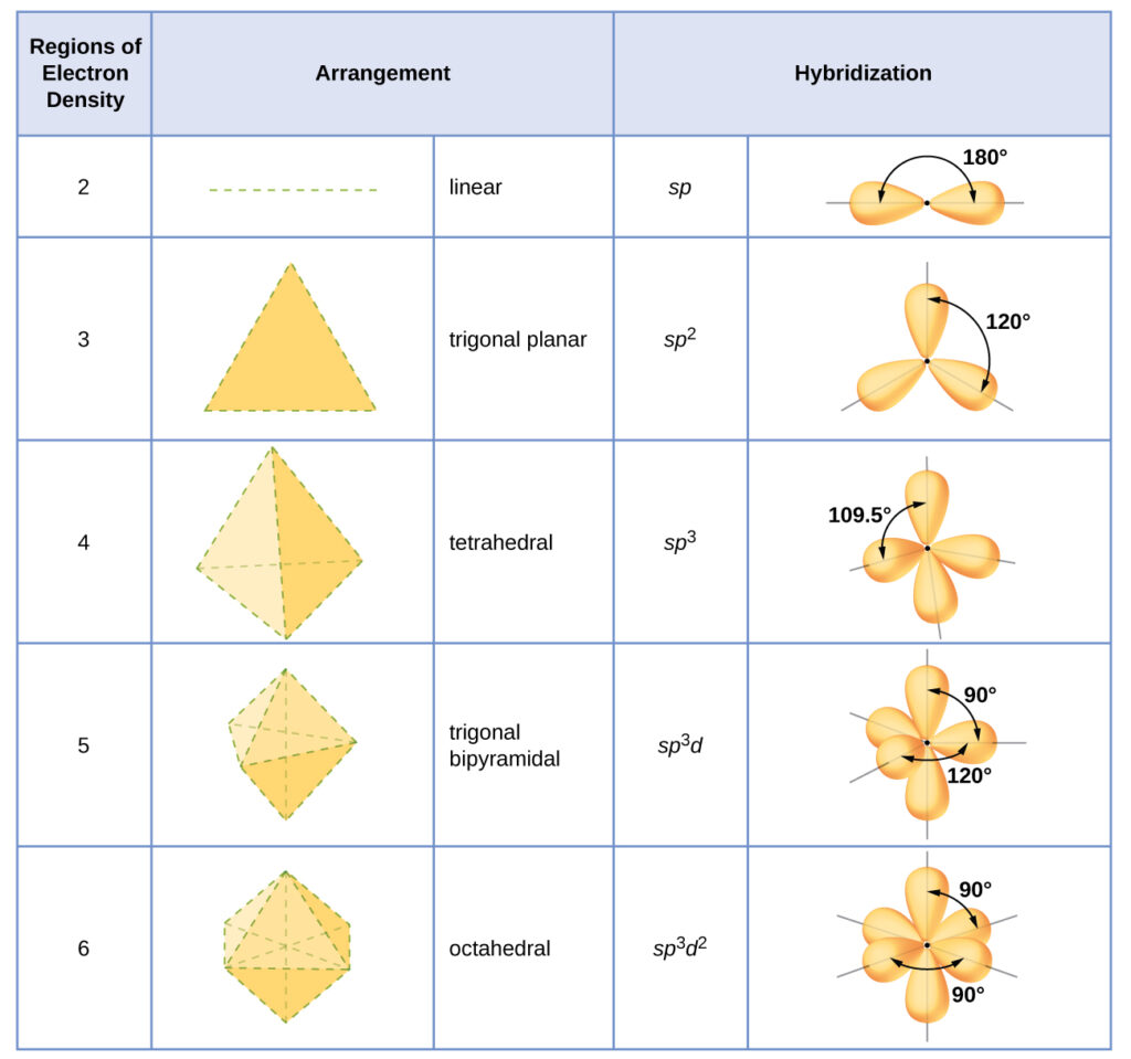
The hybridization of an atom is determined based on the number of regions of electron density that surround it. The geometrical arrangements characteristic of the various sets of hybrid orbitals are shown in the table below. These arrangements are identical to those of the electron-pair geometries predicted by VSEPR theory. VSEPR theory predicts the shapes of molecules, and hybrid orbital theory provides an explanation for how those shapes are formed. To find the hybridization of a central atom, we can use the following guidelines:

• Determine the Lewis structure of the molecule.
• Determine the number of regions of electron density around an atom using VSEPR theory, in which single bonds, multiple bonds, radicals, and lone pairs each count as one region.
• Assign the set of hybridized orbitals from the table below that corresponds to this geometry.

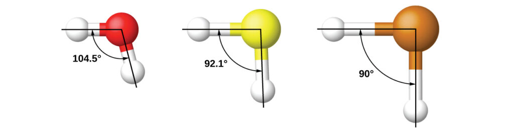
It is important to remember that hybridization was devised to rationalize experimentally observed molecular geometries. The model works well for molecules containing small central atoms, in which the valence electron pairs are close together in space. However, for larger central atoms, the valence-shell electron pairs are farther from the nucleus, and there are fewer repulsions. Their compounds exhibit structures that are often not consistent with VSEPR theory, and hybridized orbitals are not necessary to explain the observed data. For example, we have discussed the H–O–H bond angle in H 2 O, 104.5°, which is more consistent with sp 3 hybrid orbitals (109.5°) on the central atom than with 2 p orbitals (90°). Sulfur is in the same group as oxygen, and H 2 S has a similar Lewis structure. However, it has a much smaller bond angle (92.1°), which indicates much less hybridization on sulfur than oxygen. Continuing down the group, tellurium is even larger than sulfur, and for H 2 Te, the observed bond angle (90°) is consistent with overlap of the 5 p orbitals, without invoking hybridization. We invoke hybridization where it is necessary to explain the observed structures.

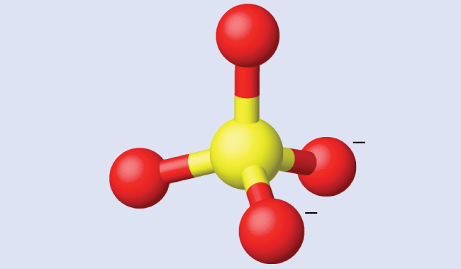
Assigning Hybridization Ammonium sulfate is important as a fertilizer. What is the hybridization of the sulfur atom in the sulfate ion, $SO_4^{2−}$?

Solution The Lewis structure of sulfate shows there are four regions of electron density. The hybridization is sp 3 .

Check Your Learning What is the hybridization of the selenium atom in SeF 4 ?

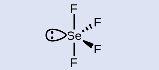
Answer: The selenium atom is sp 3 d hybridized.

Assigning Hybridization Urea, NH 2 C(O)NH 2 , is sometimes used as a source of nitrogen in fertilizers. What is the hybridization of the carbon atom in urea?

Solution The Lewis structure of urea is:

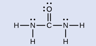
The carbon atom is surrounded by three regions of electron density, positioned in a trigonal planar arrangement. The hybridization in a trigonal planar electron pair geometry is sp 2 ( [link] ), which is the hybridization of the carbon atom in urea.

Check Your Learning Acetic acid, H 3 CC(O)OH, is the molecule that gives vinegar its odor and sour taste.

Module 8: Advanced Theories of Covalent Bonding

Hybrid atomic orbitals, learning outcomes.

• Explain the concept of atomic orbital hybridization
• Determine the hybrid orbitals associated with various molecular geometries

Figure 1. The hypothetical overlap of two of the 2 p orbitals on an oxygen atom (red) with the 1s orbitals of two hydrogen atoms (blue) would produce a bond angle of 90°. This is not consistent with experimental evidence.

Thinking in terms of overlapping atomic orbitals is one way for us to explain how chemical bonds form in diatomic molecules. However, to understand how molecules with more than two atoms form stable bonds, we require a more detailed model. As an example, let us consider the water molecule, in which we have one oxygen atom bonding to two hydrogen atoms. Oxygen has the electron configuration 1 s 2 2 s 2 2 p 4 , with two unpaired electrons (one in each of the two 2p orbitals). Valence bond theory would predict that the two O–H bonds form from the overlap of these two 2 p orbitals with the 1 s orbitals of the hydrogen atoms. If this were the case, the bond angle would be 90°, as shown in Figure 1 ( note that orbitals may sometimes be drawn in an elongated “balloon” shape rather than in a more realistic “plump” shape in order to make the geometry easier to visualize ), because p orbitals are perpendicular to each other.. Experimental evidence shows that the bond angle is 104.5°, not 90°. The prediction of the valence bond theory model does not match the real-world observations of a water molecule; a different model is needed.

Quantum-mechanical calculations suggest why the observed bond angles in H 2 O differ from those predicted by the overlap of the 1 s orbital of the hydrogen atoms with the 2 p orbitals of the oxygen atom. The mathematical expression known as the wave function, ψ , contains information about each orbital and the wavelike properties of electrons in an isolated atom. When atoms are bound together in a molecule, the wave functions combine to produce new mathematical descriptions that have different shapes. This process of combining the wave functions for atomic orbitals is called hybridization and is mathematically accomplished by the linear combination of atomic orbitals , LCAO, (a technique that we will encounter again later). The new orbitals that result are called hybrid orbitals . The valence orbitals in an isolated oxygen atom are a 2 s orbital and three 2 p orbitals. The valence orbitals in an oxygen atom in a water molecule differ; they consist of four equivalent hybrid orbitals that point approximately toward the corners of a tetrahedron (Figure 2). Consequently, the overlap of the O and H orbitals should result in a tetrahedral bond angle (109.5°). The observed angle of 104.5° is experimental evidence for which quantum-mechanical calculations give a useful explanation: Valence bond theory must include a hybridization component to give accurate predictions.

Figure 2. (a) A water molecule has four regions of electron density, so VSEPR theory predicts a tetrahedral arrangement of hybrid orbitals. (b) Two of the hybrid orbitals on oxygen contain lone pairs, and the other two overlap with the 1 s orbitals of hydrogen atoms to form the O–H bonds in H 2 O. This description is more consistent with the experimental structure.

The following ideas are important in understanding hybridization:

• Hybrid orbitals do not exist in isolated atoms. They are formed only in covalently bonded atoms.
• Hybrid orbitals have shapes and orientations that are very different from those of the atomic orbitals in isolated atoms.
• A set of hybrid orbitals is generated by combining atomic orbitals. The number of hybrid orbitals in a set is equal to the number of atomic orbitals that were combined to produce the set.
• All orbitals in a set of hybrid orbitals are equivalent in shape and energy.
• The type of hybrid orbitals formed in a bonded atom depends on its electron-pair geometry as predicted by the VSEPR theory.
• Hybrid orbitals overlap to form σ bonds. Unhybridized orbitals overlap to form π bonds.

In the following sections, we shall discuss the common types of hybrid orbitals.

sp Hybridization

The beryllium atom in a gaseous BeCl 2 molecule is an example of a central atom with no lone pairs of electrons in a linear arrangement of three atoms. There are two regions of valence electron density in the BeCl 2 molecule that correspond to the two covalent Be–Cl bonds. To accommodate these two electron domains, two of the Be atom’s four valence orbitals will mix to yield two hybrid orbitals. This hybridization process involves mixing of the valence s orbital with one of the valence p orbitals to yield two equivalent sp hybrid orbitals that are oriented in a linear geometry (Figure 3). In this figure, the set of sp orbitals appears similar in shape to the original p orbital, but there is an important difference. The number of atomic orbitals combined always equals the number of hybrid orbitals formed. The p orbital is one orbital that can hold up to two electrons. The sp set is two equivalent orbitals that point 180° from each other. The two electrons that were originally in the s orbital are now distributed to the two sp orbitals, which are half filled. In gaseous BeCl 2 , these half-filled hybrid orbitals will overlap with orbitals from the chlorine atoms to form two identical [latex]\sigma[/latex] bonds.

Figure 3. Hybridization of an s orbital (blue) and a p orbital (red) of the same atom produces two sp hybrid orbitals (purple). Each hybrid orbital is oriented primarily in just one direction. Note that each sp orbital contains one lobe that is significantly larger than the other. The set of two sp orbitals are oriented at 180°, which is consistent with the geometry for two domains.

We illustrate the electronic differences in an isolated Be atom and in the bonded Be atom in the orbital energy-level diagram in Figure 4. These diagrams represent each orbital by a horizontal line (indicating its energy) and each electron by an arrow. Energy increases toward the top of the diagram. We use one upward arrow to indicate one electron in an orbital and two arrows (up and down) to indicate two electrons of opposite spin.

Figure 4. This orbital energy-level diagram shows the sp hybridized orbitals on Be in the linear BeCl 2 molecule. Each of the two sp hybrid orbitals holds one electron and is thus half filled and available for bonding via overlap with a Cl 3 p orbital.

When atomic orbitals hybridize, the valence electrons occupy the newly created orbitals. The Be atom had two valence electrons, so each of the sp orbitals gets one of these electrons. Each of these electrons pairs up with the unpaired electron on a chlorine atom when a hybrid orbital and a chlorine orbital overlap during the formation of the Be–Cl bonds.

Any central atom surrounded by just two regions of valence electron density in a molecule will exhibit sp hybridization. Other examples include the mercury atom in the linear HgCl 2 molecule, the zinc atom in Zn(CH 3 ) 2 , which contains a linear C–Zn–C arrangement, and the carbon atoms in HCCH and CO 2 .

sp 2 Hybridization

The valence orbitals of a central atom surrounded by three regions of electron density consist of a set of three sp 2 hybrid orbitals and one unhybridized p orbital. This arrangement results from sp 2 hybridization, the mixing of one s orbital and two p orbitals to produce three identical hybrid orbitals oriented in a trigonal planar geometry (Figure 5).

Figure 5. The hybridization of an s orbital (blue) and two p orbitals (red) produces three equivalent sp 2 hybridized orbitals (purple) oriented at 120° with respect to each other. The remaining unhybridized p orbital is not shown here, but is located along the z axis.

Figure 6. This alternate way of drawing the trigonal planar sp 2 hybrid orbitals is sometimes used in more crowded figures.

Although quantum mechanics yields the “plump” orbital lobes as depicted in Figure 5, sometimes for clarity these orbitals are drawn thinner and without the minor lobes, as in Figure 6, to avoid obscuring other features of a given illustration.

We will use these “thinner” representations whenever the true view is too crowded to easily visualize.

The observed structure of the borane molecule, BH 3 , suggests sp 2 hybridization for boron in this compound. The molecule is trigonal planar, and the boron atom is involved in three bonds to hydrogen atoms (Figure 7).

Figure 7. BH 3 is an electron-deficient molecule with a trigonal planar structure.

We can illustrate the comparison of orbitals and electron distribution in an isolated boron atom and in the bonded atom in BH 3 as shown in the orbital energy level diagram in Figure 8. We redistribute the three valence electrons of the boron atom in the three sp 2 hybrid orbitals, and each boron electron pairs with a hydrogen electron when B–H bonds form.

Figure 8. In an isolated B atom, there are one 2 s and three 2 p valence orbitals. When boron is in a molecule with three regions of electron density, three of the orbitals hybridize and create a set of three sp 2 orbitals and one unhybridized 2 p orbital. The three half-filled hybrid orbitals each overlap with an orbital from a hydrogen atom to form three σ bonds in BH 3 .

Any central atom surrounded by three regions of electron density will exhibit sp 2 hybridization. This includes molecules with a lone pair on the central atom, such as ClNO (Figure 9), or molecules with two single bonds and a double bond connected to the central atom, as in formaldehyde, CH 2 O, and ethene, H 2 CCH 2 .

Figure 9. The central atom(s) in each of the structures shown contain three regions of electron density and are sp 2 hybridized. As we know from the discussion of VSEPR theory, a region of electron density contains all of the electrons that point in one direction. A lone pair, an unpaired electron, a single bond, or a multiple bond would each count as one region of electron density.

sp 3 Hybridization

The valence orbitals of an atom surrounded by a tetrahedral arrangement of bonding pairs and lone pairs consist of a set of four sp 3 hybrid orbitals . The hybrids result from the mixing of one s orbital and all three p orbitals that produces four identical sp 3 hybrid orbitals (Figure 10). Each of these hybrid orbitals points toward a different corner of a tetrahedron.

Figure 10. The hybridization of an s orbital (blue) and three p orbitals (red) produces four equivalent sp 3 hybridized orbitals (purple) oriented at 109.5° with respect to each other.

A molecule of methane, CH 4 , consists of a carbon atom surrounded by four hydrogen atoms at the corners of a tetrahedron. The carbon atom in methane exhibits sp 3 hybridization. We illustrate the orbitals and electron distribution in an isolated carbon atom and in the bonded atom in CH 4 in Figure 11. The four valence electrons of the carbon atom are distributed equally in the hybrid orbitals, and each carbon electron pairs with a hydrogen electron when the C–H bonds form.

Figure 11. The four valence atomic orbitals from an isolated carbon atom all hybridize when the carbon bonds in a molecule like CH 4 with four regions of electron density. This creates four equivalent sp 3 hybridized orbitals. Overlap of each of the hybrid orbitals with a hydrogen orbital creates a C–H σ bond.

In a methane molecule, the 1 s orbital of each of the four hydrogen atoms overlaps with one of the four sp 3 orbitals of the carbon atom to form a sigma ([latex]\sigma[/latex]) bond. This results in the formation of four strong, equivalent covalent bonds between the carbon atom and each of the hydrogen atoms to produce the methane molecule, CH 4 .

The structure of ethane, C 2 H 6, is similar to that of methane in that each carbon in ethane has four neighboring atoms arranged at the corners of a tetrahedron—three hydrogen atoms and one carbon atom (Figure 12). However, in ethane an sp 3 orbital of one carbon atom overlaps end to end with an sp 3 orbital of a second carbon atom to form a σ bond between the two carbon atoms. Each of the remaining sp 3 hybrid orbitals overlaps with an s orbital of a hydrogen atom to form carbon–hydrogen σ bonds. The structure and overall outline of the bonding orbitals of ethane are shown in Figure 12. The orientation of the two CH 3 groups is not fixed relative to each other. Experimental evidence shows that rotation around [latex]\sigma[/latex] bonds occurs easily.

Figure 12. (a) In the ethane molecule, C 2 H 6 , each carbon has four sp 3 orbitals. (b) These four orbitals overlap to form seven σ bonds.

An sp 3 hybrid orbital can also hold a lone pair of electrons. For example, the nitrogen atom in ammonia is surrounded by three bonding pairs and a lone pair of electrons directed to the four corners of a tetrahedron. The nitrogen atom is sp 3 hybridized with one hybrid orbital occupied by the lone pair. The molecular structure of water is consistent with a tetrahedral arrangement of two lone pairs and two bonding pairs of electrons. Thus we say that the oxygen atom is sp 3 hybridized, with two of the hybrid orbitals occupied by lone pairs and two by bonding pairs. Since lone pairs occupy more space than bonding pairs, structures that contain lone pairs have bond angles slightly distorted from the ideal. Perfect tetrahedra have angles of 109.5°, but the observed angles in ammonia (107.3°) and water (104.5°) are slightly smaller. Other examples of sp 3 hybridization include CCl 4 , PCl 3 , and NCl 3 .

sp 3 d and sp 3 d 2 Hybridization

To describe the five bonding orbitals in a trigonal bipyramidal arrangement, we must use five of the valence shell atomic orbitals (the s orbital, the three p orbitals, and one of the d orbitals), which gives five sp 3 d hybrid orbitals . With an octahedral arrangement of six hybrid orbitals, we must use six valence shell atomic orbitals (the s orbital, the three p orbitals, and two of the d orbitals in its valence shell), which gives six sp 3 d 2 hybrid orbitals . These hybridizations are only possible for atoms that have d orbitals in their valence subshells (that is, not those in the first or second period).

In a molecule of phosphorus pentachloride, PCl 5 , there are five P–Cl bonds (thus five pairs of valence electrons around the phosphorus atom) directed toward the corners of a trigonal bipyramid. We use the 3 s orbital, the three 3 p orbitals, and one of the 3 d orbitals to form the set of five sp 3 d hybrid orbitals (Figure 14) that are involved in the P–Cl bonds. Other atoms that exhibit sp 3 d hybridization include the sulfur atom in [latex]\text{SF}_{4}[/latex] and the chlorine atoms in [latex]\text{ClF}_{3}[/latex] and in [latex]{\text{ClF}}_{4}^{\text{+}}.[/latex] (The electrons on fluorine atoms are omitted for clarity.)

Figure 13. The three compounds pictured exhibit sp 3 d hybridization in the central atom and a trigonal bipyramid form. SF 4 and ClF 4 + have one lone pair of electrons on the central atom, and ClF 3 has two lone pairs giving it the T-shape shown.

Figure 14. (a) The five regions of electron density around phosphorus in PCl 5 require five hybrid sp 3 d orbitals. (b) These orbitals combine to form a trigonal bipyramidal structure with each large lobe of the hybrid orbital pointing at a vertex. As before, there are also small lobes pointing in the opposite direction for each orbital (not shown for clarity).

The sulfur atom in sulfur hexafluoride, [latex]\text{SF}_{6}[/latex], exhibits sp 3 d 2 hybridization. A molecule of sulfur hexafluoride has six bonding pairs of electrons connecting six fluorine atoms to a single sulfur atom (Figure 15). There are no lone pairs of electrons on the central atom. To bond six fluorine atoms, the 3 s orbital, the three 3 p orbitals, and two of the 3 d orbitals form six equivalent sp 3 d 2 hybrid orbitals, each directed toward a different corner of an octahedron. Other atoms that exhibit sp 3 d 2 hybridization include the phosphorus atom in [latex]{\text{PCl}}_{6}^{-},[/latex] the iodine atom in the interhalogens [latex]{\text{IF}}_{6}^{\text{+}}[/latex], [latex]\text{IF}_{5}[/latex], [latex]{\text{ICl}}_{4}^{-}[/latex], [latex]{\text{IF}}_{4}^{-}[/latex] and the xenon atom in [latex]\text{XeF}_{4}[/latex].

Figure 15. (a) Sulfur hexafluoride, SF 6 , has an octahedral structure that requires sp 3 d 2 hybridization. (b) The six sp 3 d 2 orbitals form an octahedral structure around sulfur. Again, the minor lobe of each orbital is not shown for clarity.

Assignment of Hybrid Orbitals to Central Atoms

The hybridization of an atom is determined based on the number of regions of electron density that surround it. The geometrical arrangements characteristic of the various sets of hybrid orbitals are shown in Figure 16. These arrangements are identical to those of the electron-pair geometries predicted by VSEPR theory. VSEPR theory predicts the shapes of molecules, and hybrid orbital theory provides an explanation for how those shapes are formed. To find the hybridization of a central atom, we can use the following guidelines:

• Determine the Lewis structure of the molecule.
• Determine the number of regions of electron density around an atom using VSEPR theory, in which single bonds, multiple bonds, radicals, and lone pairs each count as one region.
• Assign the set of hybridized orbitals from Figure 16 that corresponds to this geometry.

Figure 16. The shapes of hybridized orbital sets are consistent with the electron-pair geometries. For example, an atom surrounded by three regions of electron density is sp 2 hybridized, and the three sp 2 orbitals are arranged in a trigonal planar fashion.

Example 1: Assigning Hybridization

Ammonium sulfate is important as a fertilizer. What is the hybridization of the sulfur atom in the sulfate ion, [latex]{\text{SO}}_{4}^{2-}[/latex]?

The Lewis structure of sulfate shows there are four regions of electron density. The hybridization is sp 3 .

Check Your Learning

Example 2: Assigning Hybridization

Urea, NH 2 C(O)NH 2 , is sometimes used as a source of nitrogen in fertilizers. What is the hybridization of each nitrogen and carbon atom in urea?

The Lewis structure of urea is

The nitrogen atoms are surrounded by four regions of electron density, which arrange themselves in a tetrahedral electron-pair geometry. The hybridization in a tetrahedral arrangement is sp 3 (Figure 8.21). This is the hybridization of the nitrogen atoms in urea. The carbon atom is surrounded by three regions of electron density, positioned in a trigonal planar arrangement. The hybridization in a trigonal planar electron pair geometry is sp 2 (Figure 8.21), which is the hybridization of the carbon atom in urea.

Acetic acid, H 3 CC(O)OH, is the molecule that gives vinegar its odor and sour taste. What is the hybridization of the two carbon atoms in acetic acid?

Key Concepts and Summary

We can use hybrid orbitals, which are mathematical combinations of some or all of the valence atomic orbitals, to describe the electron density around covalently bonded atoms. These hybrid orbitals either form sigma ([latex]\sigma[/latex]) bonds directed toward other atoms of the molecule or contain lone pairs of electrons. We can determine the type of hybridization around a central atom from the geometry of the regions of electron density about it. Two such regions imply sp hybridization; three, sp 2 hybridization; four, sp 3 hybridization; five, sp 3 d hybridization; and six, sp 3 d 2 hybridization. Pi (π) bonds are formed from unhybridized atomic orbitals ( p or d orbitals).

• Why is the concept of hybridization required in valence bond theory?
• Explain why a carbon atom cannot form five bonds using sp 3 d hybrid orbitals.
• [latex]{\text{PO}}_{4}^{\text{3-}}[/latex]
• A molecule with the formula AB 3 could have one of four different shapes. Give the shape and the hybridization of the central A atom for each.

• circular S 8 molecule
• SO 2 molecule
• SO 3 molecule
• H 2 SO 4 molecule (the hydrogen atoms are bonded to oxygen atoms)
• Draw a Lewis structure.
• Predict the geometry about the carbon atom.
• Determine the hybridization of each type of carbon atom.
• What is the formula of the compound?
• Write a Lewis structure for the compound.
• Predict the shape of the molecules of the compound.
• What hybridization is consistent with the shape you predicted?
• Write a Lewis structure.
• What are the electron pair and molecular geometries of the internal oxygen and nitrogen atoms in the HNO 2 molecule?
• What is the hybridization on the internal oxygen and nitrogen atoms in HNO 2 ?

• Write Lewis structures for P 4 S 3 and the [latex]{\text{ClO}}_{3}^{-}[/latex] ion.
• Describe the geometry about the P atoms, the S atom, and the Cl atom in these species.
• Assign a hybridization to the P atoms, the S atom, and the Cl atom in these species.
• Determine the oxidation states and formal charge of the atoms in P 4 S 3 and the [latex]{\text{ClO}}_{3}^{-}[/latex] ion.

• Write Lewis structures for NF 3 and PF 5 . On the basis of hybrid orbitals, explain the fact that NF 3 , PF 3 , and PF 5 are stable molecules, but NF 5 does not exist.
• In addition to NF 3 , two other fluoro derivatives of nitrogen are known: N 2 F 4 and N 2 F 2 . What shapes do you predict for these two molecules? What is the hybridization for the nitrogen in each molecule?

1. Hybridization is introduced to explain the geometry of bonding orbitals in valance bond theory.

3. There are no d orbitals in the valence shell of carbon.

5. trigonal planar, sp 2 , trigonal pyramidal (one lone pair on A) sp 3 , T-shaped (two lone pairs on A sp 3 d , or (three lone pair on A) sp 3 d 2

7. The Lewis structures and predicted molecular geometries are as follows:

9. The answers are as follows:

• [latex]\dfrac{\text{77.55 g}}{\text{131.29 g}{\text{ mol}}^{-1}}=0.5907\text{ mol}[/latex]
• [latex]\dfrac{\text{22.45 g}}{\text{18.998 g}{\text{ mol}}^{-1}}=\text{1.182 mol}[/latex]

Find the ratio by dividing by the smaller value.

• [latex]\dfrac{1.182}{0.5907}=2.001[/latex]

• There are 22 electrons, 16 of which are used in the bond, leaving six electrons in the three pairs of unbonded electrons centered about the Xe. These unshared electrons are in a trigonal planar shape with the bonding pairs above and below the plane. Therefore, XeF 2 is linear.
• sp 3 d hybridization is consistent with the linear shape.

11. The answers are as follows:

• P atoms, trigonal pyramidal; S atoms, bent, with two lone pairs; Cl atoms, trigonal pyramidal;
• Hybridization about P, S, and Cl is, in all cases, sp 3 ;
• Oxidation states P +1, S [latex]-1\frac{1}{3},[/latex] Cl +5, O –2. Formal charges: P 0; S 0; Cl +2: O –1

13. Phosphorus and nitrogen can form sp 3 hybrids to form three bonds and hold one lone pair in PF 3 and NF 3 , respectively. However, nitrogen has no valence d orbitals, so it cannot form a set of sp 3 d hybrid orbitals to bind five fluorine atoms in NF 5 . Phosphorus has d orbitals and can bind five fluorine atoms with sp 3 d hybrid orbitals in PF 5 .

hybrid orbital:  orbital created by combining atomic orbitals on a central atom

hybridization:  model that describes the changes in the atomic orbitals of an atom when it forms a covalent compound

sp hybrid orbital:  one of a set of two orbitals with a linear arrangement that results from combining one s and one p orbital

sp 2 hybrid orbital:  one of a set of three orbitals with a trigonal planar arrangement that results from combining one s and two p orbitals

sp 3 hybrid orbital:  one of a set of four orbitals with a tetrahedral arrangement that results from combining one s and three p orbitals

sp 3 d hybrid orbital:  one of a set of five orbitals with a trigonal bipyramidal arrangement that results from combining one s , three p , and one d orbital

sp 3 d 2 hybrid orbital:  one of a set of six orbitals with an octahedral arrangement that results from combining one s , three p , and two d orbitals

• Chemistry 2e. Provided by : OpenStax. Located at : https://openstax.org/ . License : CC BY: Attribution . License Terms : Access for free at https://openstax.org/books/chemistry-2e/pages/1-introduction

• IIT JEE Study Material

Hybridization

Hybridization , in Chemistry, is defined as the concept of mixing two atomic orbitals to give rise to a new type of hybridized orbitals. This intermixing usually results in the formation of hybrid orbitals having entirely different energy, shapes, etc. The atomic orbitals of the same energy level mainly take part in hybridization. However, both fully-filled and half-filled orbitals can also take part in this process, provided they have equal energy.

Download Complete Chapter Notes of Chemical Bonding and Molecular Structure Download Now

On the other hand, we can say that the concept of hybridization is an extension of the valence bond theory, and it helps us to understand the formation of bonds, bond energies and bond lengths.

Table of Contents

• Key Features

sp Hybridization

Sp 2  hybridization, sp 3  hybridization, sp 3 d hybridization.

• sp 3 d2 Hybridization

What Is Hybridization?

Redistribution of the energy of orbitals of individual atoms to give orbitals of equivalent energy happens when two atomic orbitals combine to form a hybrid orbital in a molecule. This process is called hybridization .  During the process of hybridization, the atomic orbitals of comparable energies are mixed together and mostly involves the merging of two ‘s’ orbitals or two ‘p’ orbitals or the mixing of an ‘s’ orbital with a ‘p’ orbital, as well as ‘s’ orbital with a ‘d’ orbital. The new orbitals, thus formed, are known as hybrid orbitals.  More significantly, hybrid orbitals are quite useful in explaining atomic bonding properties and molecular geometry.

Let us have a quick look at the example of a carbon atom. This atom forms 4 single bonds wherein the valence-shell s orbital mixes with 3 valence-shell p orbitals. This combination leads to the formation of 4 equivalent sp 3 mixtures. They will have a tetrahedral arrangement around the carbon, which is bonded to 4 different atoms.

Hybridization Video Lesson

⇒ Also Read

• Chemical Bonding
• Molecular Orbital Theory

Key Features of Hybridization

• Atomic orbitals with equal energies undergo hybridization.
• The number of hybrid orbitals formed is equal to the number of atomic orbitals mixed.
• It is not necessary that all the half-filled orbitals must participate in hybridization. Even completely filled orbitals with slightly different energies can also participate.
• Hybridization happens only during the bond formation and not in an isolated gaseous atom.
• The shape of the molecule can be predicted if the hybridization of the molecule is known.
• The bigger lobe of the hybrid orbital always has a positive sign, while the smaller lobe on the opposite side has a negative sign.

Try this: Give the hybridization states of each of the carbon atoms in the given molecule.

• H 2 C = CH – CN
• HC ≡ C − C ≡ CH
• H 2 C = C = C = CH 2

Types of Hybridization

Based on the types of orbitals involved in mixing, the hybridization can be classified as sp 3 , sp 2 , sp, sp 3 d, sp 3 d 2 and sp 3 d 3 . Let us now discuss the various types of hybridization, along with their examples.

sp hybridization is observed when one s and one p orbital in the same main shell of an atom mix to form two new equivalent orbitals. The new orbitals formed are called  sp hybridized orbitals.  It forms linear molecules with an angle of 180°.

• This type of hybridization involves the mixing of one ‘s’ orbital and one ‘p’ orbital of equal energy to give a new hybrid orbital known as an sp hybridized orbital.
• The sp hybridization is also called diagonal hybridization.
• Each sp hybridized orbital has an equal amount of s and p characters – 50% s and 50% p characters.

Examples of sp Hybridization:

• All compounds of beryllium , like BeF 2 , BeH 2,  BeCl 2
• All compounds of a carbon-containing triple bond, like C 2 H 2 .

sp 2  hybridization  is observed when one s and two p orbitals of the same shell of an atom mix to form 3 equivalent orbitals. The new orbitals formed are called  sp 2  hybrid orbitals. 

• sp 2 hybridization is also called trigonal hybridization.
• It involves the mixing of one ‘s’ orbital and two ‘p’ orbitals of equal energy to give a new hybrid orbital known as sp 2 .
• A mixture of s and p orbital formed in trigonal symmetry and is maintained at 120 0 .
• All three hybrid orbitals remain in one plane and make an angle of 120° with one another. Each of the hybrid orbitals formed has a 33.33% ‘s’ character and 66.66% ‘p’ character.
• The molecules in which the central atom is linked to 3 atoms and is sp2 hybridized have a triangular planar shape.

Examples of sp 2  Hybridization

• All the compounds of Boron, i.e., BF 3 and  BH 3
• All the compounds of carbon, containing a carbon-carbon double bond, Ethylene (C 2 H 4 )

When one ‘s’ orbital and 3 ‘p’ orbitals belonging to the same shell of an atom mix together to form four new equivalent orbitals, the type of hybridization is called a tetrahedral hybridization or sp 3 . The new orbitals formed are called  sp 3  hybrid orbitals.

• These are directed towards the four corners of a regular tetrahedron and make an angle of 109°28’ with one another.
• The angle between the sp3 hybrid orbitals is 109.28 0
• Each sp 3  hybrid orbital has 25% s character and 75% p character.
• Examples of sp 3 hybridization are ethane (C 2 H 6 ) and methane.

sp 3 d hybridization involves the mixing of 1s orbital,  3p orbitals and 1d orbital to form 5 sp 3 d hybridized orbitals of equal energy. They have trigonal bipyramidal geometry.

• The mixture of s, p and d orbital forms trigonal bipyramidal symmetry.
• Three hybrid orbitals lie in the horizontal plane inclined at an angle of 120° to each other, known as the equatorial orbitals.
• The remaining two orbitals lie in the vertical plane at 90 degrees plane of the equatorial orbitals, known as axial orbitals.
• Example: Hybridization in phosphorus pentachloride (PCl 5 )

sp 3 d 2  Hybridization

• sp 3 d 2 hybridization has 1s, 3p and 2d orbitals, that undergo intermixing to form 6 identical sp 3 d 2  hybrid orbitals.
• These 6 orbitals are directed towards the corners of an octahedron.
• They are inclined at an angle of 90 degrees to one another.

Frequently Asked Questions on Hybridization

What are the different types of hybridization.

Based on the nature of the mixing orbitals, hybridization can be classified in the following ways:

• sp hybridization (beryllium chloride, acetylene)
• sp 2 hybridization (boron trichloride, ethylene)
• sp 3 hybridization (methane, ethane)
• sp 3 d hybridization (phosphorus pentachloride)
• sp 3 d 2 hybridization (sulphur hexafluoride)
• sp 3 d 3 hybridization (iodine heptafluoride)

⇒ Know more about VSEPR theory, its postulates and limitations

Among sp, sp 2 and sp 3 , which hybrid orbital is more electronegative?

The percentage of s character in sp, sp 2 and sp 3 hybridized carbon is 50%, 33.33%, and 25%, respectively.

⇒ Also Read:

• Hydrogen Bonding
• Covalent Bond

Due to the spherical shape of the s orbital, it is attracted evenly by the nucleus from all directions. Therefore, a hybrid orbital with more s-character will be closer to the nucleus, and thus more electronegative. Hence, the sp hybridized carbon is more electronegative than sp 2 and sp 3 .

Why is the hybrid orbital during hybridization better than its parent atoms?

The reason why a hybrid orbital is better than its parents is as follows:

• Parent s: because it is directional, unlike the s orbital.
• Parent p: because it has lower energy than p orbital.

What are hybrid orbitals?

Hybrid orbitals can be defined as the combination of standard atomic orbitals resulting in the formation of new atomic orbitals.

⇒ Check: Fajan’s Rule and Its Postulates

During hybridization, the hybrid orbitals possess different geometry of orbital arrangement and energies than the standard atomic orbitals. Also, the orbital overlap minimises the energy of the molecule. The degenerate hybrid orbitals formed from the standard atomic orbitals are as listed:

• 1s and 1 p: sp orbitals
• 1s and 2p: sp 2 orbitals
• 1s and 3p: sp 3 orbitals
• 1s, 3p, and 1d: sp 3 d orbitals
• 1s, 3p, and 2d: sp 3 d 2 orbitals

What is the difference between sp, sp 2 and sp 3 hybridization?

The sp hybridization occurs due to the mixing of one s and one p atomic orbital, the sp 2 hybridization is the mixing of one s and two p atomic orbitals, and the sp 3 hybridization is the mixing of one s and three p atomic orbitals.

What is the percentage of s and p characters in sp, sp 2 and sp 3 hybrid orbitals?

The percentage of s and p characters in sp, sp 2 and sp 3 hybrid orbitals is,

Sp: s characteristic 50% and p characteristic 50%

Sp 2 : s characteristic 33.33% and p characteristic 66.66%

Sp 3 : s characteristic 25% and p characteristic 75%

Explain the five basic shapes of hybridization.

The five basic shapes of hybridization are linear, trigonal planar, tetrahedral, trigonal bipyramidal and octahedral.

The geometry of the orbital arrangement is as follows:

• Linear: Two electron groups are involved resulting in sp hybridization; the angle between the orbitals is 180°.
• Trigonal planar: Three electron groups are involved resulting in sp 2 hybridization, and the angle between the orbitals is 120°.
• Tetrahedral: Four electron groups are involved resulting in sp 3 hybridization, and the angle between the orbitals is 109.5°.
• Trigonal bipyramidal: Five electron groups are involved resulting in sp 3 d hybridization; the angle between the orbitals is 90°, 120°.
• Octahedral: Six electron groups are involved resulting in sp 3 d 2 hybridization, and the angle between the orbitals is 90°.

Explain the sp3 hybridization in methane.

The 2s and all the three (3p) orbitals of carbon hybridize to form four sp 3 orbitals. These hybrid orbitals bond with four atoms of hydrogen through sp3-s orbital overlap resulting in CH 4 (methane). The geometry of orbital arrangement due to the minimum electron repulsion is tetrahedral.

The amide molecule looks like the sp 3 hybridized, but it is sp 2 . Why?

The general process of hybridization will change if the atom is either enclosed by two or more p orbitals or it has a lone pair to jump into a p orbital. Therefore, in the case of an amide molecule, the lone pair goes into a p orbital to have 3 adjacent parallel p orbitals (conjugation).

What results in the sp, sp 2 and sp 3 hybridization?

The sp and sp 2 hybridization results in two and one unhybridized p orbitals, respectively, whereas in the sp3 hybridization, there are no unhybridized p orbitals.

Explain the difference between molecular and hybrid orbitals.

The interactions between the atomic orbitals of two different atoms result in molecular orbitals, whereas when the atomic orbitals of the same atom interact, they form hybrid orbitals.

Put your understanding of this concept to test by answering a few MCQs. Click ‘Start Quiz’ to begin!

Select the correct answer and click on the “Finish” button Check your score and answers at the end of the quiz

Visit BYJU’S for all JEE related queries and study materials

Your result is as below

Request OTP on Voice Call

Leave a Comment Cancel reply

Your Mobile number and Email id will not be published. Required fields are marked *

Post My Comment

very useful

Thanks for such wonderful knowledge

Excellent knowledge thankyou

Very useful

Very helpful and easy to understand

Thanks for such good information

I have been interested with your presentation

• Share Share

Register with Aakash BYJU'S & Download Free PDFs

Register with byju's & watch live videos.

Pathways to Chemistry

Chemistry for college, middle and high school, homeschooled students, teachers and parents, solutions for hybridization exercises.

Exercise 1. Which is a stronger bond, a σ or π bond? The sigma bond, σ, is stronger.

Back to Hybridization of Orbitals

Exercise 2. What hybridization is expected for the underlined atoms in the following?

a) C H 3 –

First, we draw the Lewis structure.

The carbon is sp 3 hybridized.

b) C H 3 S H

Both the carbon and sulfur atoms are sp 3 hybridized.

c) H 2 C =O

The carbon atom is sp 2 hybridized.

The boron atom is sp 2 hybridized.

Exercise 3. What is the hybridization of Br in BrO 2 – ?

Exercise 4. What is the hybridization of both N atoms in H 2 N 2 ?

Exercise 5. Describe the overlap of orbitals for H 3 C-CN as well as the hybridization of the two carbon atoms.

Draw the Lewis structure.

The first carbon is sp 3 hybridized. The second carbon is sp hybridized. Carbon and hydrogen bond via overlap of a hybridized sp 3 orbital on carbon with a 1s orbital of hydrogen. The C-C bond is due to the overlap of a hybridized sp 3 orbital on the first carbon with an sp hybridized orbital of the second carbon. The carbon and nitrogen bond is due to the overlap of an sp hybridized orbital on the carbon with an sp hybridized orbital on nitrogen.

Exercise 6. Describe the overlap of orbitals in HCCCl. Use hybridization schemes.

Both carbons are sp hybridized. The carbon and hydrogen are bonded due to the overlap of a 1s oribtal of hydrogen and a hybridized sp orbital of carbon. The carbon and chlorine bond is due to the overlap of a 3p orbital in chlorine and a hybridized sp orbital of carbon.

Exercise 7. The following shows how the atoms are connected in the amino acid leucine.

Draw a Lewis structure and then determine the hybridization of all non-terminal atoms.

Carbons 1, 2, 3, and 4 are sp 3 hybridized. Carbon 5 is sp 2 hybridized. The oxygens are sp 3 hybridized, and the nitrogen is sp 3 hybridized.

Leave a Reply Cancel reply

Your email address will not be published. Required fields are marked *

Talk to our experts

1800-120-456-456

Hybridisation - JEE Important Topic

• Hybridisation

A Brief Introduction to Hybridisation

In Chemistry, hybridisation is the combination of two or more atomic orbitals with different energies to form a new atomic orbital with a lower energy. The term "hybridisation" was first used in 1898 by British chemist Frederick Crick. 

The concept of hybridisation explains the bonding properties of molecules and atoms. It is important in determining the shapes of molecules and their reactivity. In organic chemistry, hybridisation is also used to describe the sharing of electrons between atoms in a covalent bond. So read on to learn more about this fascinating concept.

What is Hybridisation?

Hybridisation of atoms refers to the process of combining two atoms together to form a new molecule. Hybridisation can occur spontaneously or as part of a chemical reaction.

Hybridisation involves taking two atoms from different elements and combining them to create a new substance. This process can happen spontaneously or be catalysed by another agent, such as heat or light. 

Important Features of Hybridisation

Hybridisation is a process of mixing two or more atomic orbitals with each other to form new hybrid orbitals.

The number of hybrid orbitals formed is equal to the number of atomic orbitals involved in the process.

The energy of these new hybrid orbitals is lower than that of the original atomic orbitals. This results in a decrease in overall energy for the atom, making it more stable.

The shapes of molecules can be predicted by looking at the types of orbitals involved in their formation. For example, if two sp orbitals form a molecule, it will be linear in shape (like $C{{O}_{2}}$).

Types of Hybridisation

The term 'hybridisation' refers to the process of combining two or more atomic orbitals into new orbitals with different shapes and energies. The resulting orbitals are called 'hybrids'. One type of hybridisation that can occur is called 'diagonal hybridisation'. This occurs when two orbitals on the same atom are combined to form a single hybrid orbital. The most common example of this is when two p-orbitals combine to form a single sp-hybrid orbital.

The resulting hybrids have properties that are intermediate between those of the original orbitals. For example, an sp-hybridised orbital has one lobe that is larger than the other, and its energy is somewhere between that of an s-orbital and a p-orbital.

There are three types of hybridisation: sp 3 , sp 2 and sp. The type of hybridisation depends on the number of valence orbitals being combined. 

sp: This involves the combination of two orbitals - one s orbital and one p orbital. The resulting molecular orbital has 50% s character and 50% p character. Diagonal hybridisation of atom is present in acetylene (${{C}_{2}}{{H}_{2}}$).

SP Hybridisation

sp 2 : This type involves the combination of three orbitals - one s orbital and two p orbitals. The resulting molecular orbital has 33% s character and 67% p character. Examples include ethene (${{C}_{2}}{{H}_{4}}$) and propene ($C{}_{3}{{H}_{6}}$). 

$s{{p}^{2}}$ Hybridisation

sp 3 : This type of hybridization occurs when four orbitals are involved in bonding - one s orbital and three p orbitals. The resulting molecular orbital has 25% s character and 75% p character. Examples include methane ($C{{H}_{4}}$) and ethane (${{C}_{2}}{{H}_{6}}$). 

$s{{p}^{3}}$ Hybridisation

sp 3 d : This type of hybridisation occurs when four orbitals are involved in bonding - one s orbital, three p orbitals and one d orbitals. One example of sp 3 d is pcl 5 .

$s{{p}^{3}}d$ Hybridisation

sp 3 d 2 : This type of hybridisation occurs when four orbitals are involved in bonding - one s orbital, three p orbitals and two d orbitals. They are inclined at an angle of 90 degrees to one another.

sp 3 d 2 Hybridisation

Shapes of Hybridisation

Linear: The sp hybridisation is caused by the interaction of two-electron groups; the orbital angle is 180°.

Trigonal planar: Three electron groups are involved, resulting in $s{{p}^{2}}$ hybridisation; the orbitals are 120° apart.

Tetrahedral: Four electron groups are involved, resulting in $s{{p}^{3}}$ hybridisation; the orbital angle is 109.5°.

Trigonal bipyramidal: Five electron groups are involved, resulting in $s{{p}^{3}}d$ hybridisation; the orbital angles are 90° and 120°.

Octahedral: Six electron groups are involved, resulting in $s{{p}^{3}}{{d}^{2}}$ hybridisation; the orbitals are 90° apart.

Define Hybridisation of Atom

An atom is the basic unit of an element that consists of a nucleus composed of protons and neutrons with electrons orbiting around this nucleus. The term 'hybridisation' refers to the process whereby atoms combine to form molecules by sharing electrons. This results in the formation of new atomic orbitals which are a combination of the original orbitals. The type of hybridisation that occurs depends on the number of valence electrons that each atom has.

There are various hybridisation atom examples and the most common type of hybridisation is known as sp3 hybridisation. This involves the mixing or 'hybridising' of one s orbital and three p orbitals to form four new atomic orbitals, each with a different shape. These four orbitals can then accommodate a total of eight electrons, which is the maximum number possible for this type of hybridisation. The resulting molecule has a tetrahedral structure with bond angles of 109.5 degrees. 

Examples of molecules that undergo sp3 hybridisation include methane ($C{{H}_{4}}$), ethane (${{C}_{2}}{{H}_{6}}$), propane (${{C}_{3}}{{H}_{8}}$) and butane (${{C}_{4}}{{H}_{10}}$). All these molecules have a central carbon atom that is bonded to four hydrogen atoms, resulting in a stable molecule with no lone pairs. Other types of hybridisation include $s{{p}^{2}}$ and sp hybridisation.

How to Find the Hybridisation of an Atom?

Rules for finding the type of hybridisation.

To understand the type of hybridisation in a compound or an ion, the following rules must be followed:

Calculate the total number of valence electrons.

Calculate the number of duplex or octet OR.

Determine the number of lone pairs of electrons.

Number of used orbital = Number of duplex or octet + Number of lone pairs of electrons.

If there is no lone pair of electrons then the geometry of orbitals and molecules is different.

Summary 

The hybridisation of atoms refers to the process of combining two atoms together to form a new molecule. Hybridisation can occur spontaneously or as part of a chemical reaction. It involves taking two atoms from different elements and combining them to create a new substance. The term "hybridisation" was first used in 1898 by British chemist Frederick Crick. There are three types of hybridisation: $s{{p}^{3}}$, $s{{p}^{2}}$, and sp. The type of hybridisation depends on the number of valence orbitals being combined. 

FAQs on Hybridisation - JEE Important Topic

1. What is hybridisation? 

In Chemistry, hybridisation is the concept of mixing atomic orbitals into new hybrid orbitals (with different energies, shapes, etc., than the original atomic orbitals) suitable for the pairing of electrons to form chemical bonds in valence bond theory. Hybridisation is possible because the orbitals of an atom are not always symmetrical with respect to the nucleus of the atom (the centre of electron density) and thus can sometimes interact more strongly with some atoms or groups of atoms than others. Hybridisation often occurs when an atom engages in covalent bonding with another atom (or group of atoms). The resulting orbital shapes are very important in understanding many properties, such as acidity/basicity, reactivity, solubility, etc. that determine how molecules behave both individually and in reactions with each other.

2. Why do we need to study hybridisation? 

We need to study hybridisation because it helps us understand molecular structure and behaviour. Many physical and chemical properties depend on the shape of molecules, which in turn depends on the arrangement of electrons around the nuclei. The way electrons are arranged in orbitals also affects things like reactivity and bond strength. By understanding how hybridisation works, we can better predict how molecules will behave in various situations.

3. What types of orbitals can be involved in hybridisation? 

Generally speaking, any type of orbital can be involved in hybridisation - s-orbitals, p-orbitals, d-orbitals, and f-orbitals. The most common type of hybridisation involves sp-orbitals (a mix between an s-orbital and a p-orbital), but there are many other possibilities too.

An official website of the United States government

The .gov means it’s official. Federal government websites often end in .gov or .mil. Before sharing sensitive information, make sure you’re on a federal government site.

The site is secure. The https:// ensures that you are connecting to the official website and that any information you provide is encrypted and transmitted securely.

• Publications
• Account settings

Preview improvements coming to the PMC website in October 2024. Learn More or Try it out now .

• Advanced Search
• Journal List
• Plant Physiol
• v.173(1); 2017 Jan

Hybridization in Plants: Old Ideas, New Techniques [OPEN]

Hybridization impacts the evolution of lineages through many mechanisms, including adaptive introgression, transgressive segregation, and hybrid speciation.

Hybridization has played an important role in the evolution of many lineages. With the growing availability of genomic tools and advancements in genomic analyses, it is becoming increasingly clear that gene flow between divergent taxa can generate new phenotypic diversity, allow for adaptation to novel environments, and contribute to speciation. Hybridization can have immediate phenotypic consequences through the expression of hybrid vigor. On longer evolutionary time scales, hybridization can lead to local adaption through the introgression of novel alleles and transgressive segregation and, in some cases, result in the formation of new hybrid species. Studying both the abundance and the evolutionary consequences of hybridization has deep historical roots in plant biology. Many of the hypotheses concerning how and why hybridization contributes to biological diversity currently being investigated were first proposed tens and even hundreds of years ago. In this Update, we discuss how new advancements in genomic and genetic tools are revolutionizing our ability to document the occurrence of and investigate the outcomes of hybridization in plants.

In natural populations, hybridization can act in opposition to divergence, introduce adaptive variation into a population, drive the evolution of stronger reproductive barriers, or generate new lineages. Hybridization is purposefully employed in the breeding of domesticated plants to take advantage of transient hybrid vigor, move desirable variation among lineages, and generate novel phenotypes. With the advent of next-generation sequencing and the availability of genomic data sets has come a tide of interest in hybridization and introgression. This includes the development of methods for detecting gene flow and a steadily growing set of empirical studies of natural hybridization (for review, see Payseur and Rieseberg, 2016 ) as well as a shift toward thinking of phylogenies as reticulate webs rather than strictly bifurcating trees ( Mallet et al., 2016 ). One reason for this trend is that genomic data are particularly well suited to address the problem of detecting gene flow. Another is the growing recognition that hybridization is widespread and may have significant evolutionary consequences, a long-held belief about plants that is increasingly extended to animals ( Mallet, 2005 ; Arnold, 2006 ; Abbott et al., 2013 ; Vallejo-Marín and Hiscock, 2016 ).

The study of hybridization in plants has a rich history. Verne Grant (1981) noted that much of the historical work on hybridization in plants could be partitioned into cataloging the frequency of hybridization and exploring the evolutionary consequences of hybridization. To this day, our research on hybridization still focuses on these two themes. In plants, scientific identification of hybrids is thought to have begun in 1716, when Cotton Mather described corn/maize ( Zea mays ) and squash ( Cucurbita spp.) plants as being of hybrid origin ( Zirkle, 1934 ). Around the same time Thomas Fairchild produced what was likely the first intentional wild plant hybrid between two Dianthus species ( Zirkle, 1934 ). Over the next 300 years, botanists including J.E. Smith (1804) , Wilhelm Olbers Focke (1881) , and Leonard Cockayne (1923) made notable efforts to catalog natural hybridization ( Anderson and Stebbins, 1954 ; Stebbins, 1959 ). Until the advent of molecular data, hybrids had to be identified by phenotypic comparisons, a practice that was eventually formalized into the hybrid index ( Anderson, 1949 ).

Joseph Gottlieb Kölreuter (1766) is credited with the first rigorous investigations of the consequences of hybridization, showing, for instance, that early-generation hybrids tend to be phenotypically intermediate between parents but may be more luxuriant, while later-generation hybrids more closely resemble parental forms. Following Kölreuter (1766) , many botanists have introduced or developed major hypotheses regarding the consequences of hybridization, including work on heterosis ( Jones, 1917 ; East, 1936 ), transgressive segregation and adaptive introgression ( Lotsy, 1916 ), and hybrid speciation ( Winge, 1917 ; Müntzing, 1930 ). Finally, Edgar Anderson (1949) and G. Ledyard Stebbins (1950) both synthesized and developed many of these ideas, making major botanical contributions to the modern synthesis.

Our goal is to draw connections between the conception and development of ideas in plant hybridization and the recent and future work in these areas. This Update is not meant to be an exhaustive review of the literature; rather, we hope to present a handful of research areas that combine rich histories of botanical and evolutionary thought with exciting recent advancements. In particular, we consider the ways in which genomic data have changed how we think about hybridization in plants and highlight areas that we believe are especially accessible to genomic study. We also recognize that, while genomic data provide previously inaccessible insight into the evolutionary history of plant populations, they are most powerful when combined with classical experiments (i.e. to determine the strength of selection in the field or the molecular function of a particular allele).

IDENTIFYING HYBRIDIZATION

One of the greatest achievements of genomics is revealing the fundamental role of hybridization in shaping the history of life on earth. In spite of some disagreement regarding the definition of hybridization ( Box 1 ), it is clear that a significant proportion of plant and animal taxa have experienced hybridization and introgression ( Mallet, 2005 ). The concept of genetic introgression, defined as the movement of genetic material between parental types through the production of and mating with hybrids ( Grant, 1981 ), predates the genomic era and was founded upon observations of increased phenotypic variation in areas of contact between plant species ( Du Rietz, 1930 ; Marsden-Jones, 1930 ). Introgression was formerly inferred by using hybrid indices and pictorialized scatter diagrams, which scored individuals from putative hybrid populations based on the similarity to phenotypes of parental forms ( Anderson, 1949 ; Grant, 1981 ). These indices are based on the idea that parental phenotypes are recombined in hybrids and that the proportion and distribution of these phenotypes will reflect the amount and nature of introgression. However, Anderson (1948) lamented that “Gene flow from one species to another may go far beyond any point which could be detected by ordinary morphological techniques. We shall not be able to assess the real importance of introgression until we can study genetically analyzed species in the field and determine the actual spread of certain marker genes.”

As predicted by Anderson (1948) , analyses of sequence divergence, haplotype structure, and allele frequency distributions in genomic data have fundamentally improved our ability to detect hybridization and even identify introgressed loci ( Rieseberg et al., 1993 ; Payseur and Rieseberg, 2016 ).

The evolutionary history of a population is reflected in the genetic variation of its genomes. Model-based methods are widely used to infer global (genome-average) and local (locus-specific) ancestry from population variation data ( Gompert and Buerkle, 2013 ; Liu et al., 2013 ). For example, the program STRUCTURE uses a hierarchical Bayesian model to identify subpopulations and estimate global ancestry for each sampled individual based on allele frequency data ( Pritchard et al., 2000 ; Porras-Hurtado et al., 2013 ) and has been extended to estimate locus-specific ancestry ( Falush et al., 2003 ). Maximum likelihood-based programs, like ADMIXTURE ( Alexander et al., 2009 ), allow for less computationally intensive estimates of genetic ancestry. Model-based methods that infer locus-specific ancestry ( Falush et al., 2003 ; Sankararaman et al., 2008 ; Paşaniuc et al., 2009 ; Price et al., 2009 ) are particularly useful for detecting hybridization and introgression without requiring a priori assignment of samples into different populations and can be used on taxa without a reference genome ( Vähä and Primmer, 2006 ; Porras-Hurtado et al., 2013 ). For instance, such analyses have been used to identify crop-wild introgression in chicory ( Cichorium intybus ) and maize ( Kiær et al., 2009 ; Hufford et al., 2013 ). However, many of these model-based analyses may have difficulty distinguishing between different evolutionary histories, as they do not account for incomplete lineage sorting ( ILS ) or estimate the timing of introgression ( Falush et al., 2016 ).

Independent mutations accumulate in the genomes of reproductively isolated taxa; therefore, the amount and pattern of genetic differences between species reveal the relative time of divergence between them. Phylogenetics-based analyses utilize this property of genetic variation to infer hybridization and introgression based on gene tree discordance and relative divergence patterns. Specifically, a sequence that is introgressed is expected to show less divergence than is expected based on the phylogenetic relationship of two lineages. A phylogenetic analysis of such loci will be discordant with the species tree ( Fig. 1A ). But introgression is not the only phenomenon that can cause discrepancies between gene trees. The persistence of ancestral polymorphism after the divergence of two species can produce phylogenetic signals that differ from the species tree. This phenomenon, known as ILS , produces a signal of incongruence that, in some ways, mimics introgression ( Fig. 1A ).

Differentiating between introgression and ILS . A, Individual gene trees may be incongruent with the species tree (outlined in black) due to either ILS (purple) or introgression (orange). Genetic divergence, as indicated by total branch length, between taxa 2 and 3 is predicted to be shorter under introgression than ILS . B, The ABBA-BABA test is used to detect an excess of one pattern of discordance relative to the other in four taxon phylogenies (three ingroup taxa and an outgroup) by comparing counts of allele patterns at polymorphic sites that differ from the species tree (outlined in black). If the star symbol represents mutation from ancestral A alleles to derived B alleles, then in this example, incongruent ABBA allele patterns are due to either introgression (orange) or ILS (purple). BABA allele patterns are due to ILS alone. An equal number of incongruent ABBA and BABA allele patterns are expected under ILS alone; therefore, a significant excess of ABBA allele patterns is consistent with a history of introgression.

Several phylogenomic analyses have been developed to infer introgression in spite of ILS . The ABBA-BABA test is currently the most widely used and is based on counts of ancestral (A) and derived (B) alleles in sets of four samples with known phylogenetic relationships (i.e. three ingroups and an outgroup). Two allele patterns, ABBA and BABA, are incongruent with the species tree BBAA and can be used to infer introgression ( Green et al., 2010 ). Under ILS , the two patterns should be equally frequent; therefore, a significant excess of one pattern over the other (as evaluated with Patterson’s D statistic) is indicative of introgression ( Fig. 1B ). These analyses have been used to successfully detect ancient and recent introgression in spite of high levels of ILS ( Pease et al., 2016 ; Ru et al., 2016 ).

Another approach to infer reticulate evolutionary histories is to model phylogenetic networks in which introgression is represented by nodes connecting hybridizing species in a phylogenetic tree ( Bapteste et al., 2013 ; Hahn and Nakhleh, 2016 ; Mallet et al., 2016 ). These methods have proven particularly useful for inferring the timing, magnitude, and direction of gene flow ( Than et al., 2008 ; Solís-Lemus and Ané, 2016 ).

Because recombination breaks apart haplotypes over time, recent introgression is expected to generate long-shared haplotype blocks between hybridizing species, a pattern that is not predicted under ILS . Therefore, the distribution of haplotype block sizes can be used to infer introgression ( Pool and Nielsen, 2009 ; Gravel, 2012 ; Mailund et al., 2012 ; Harris and Nielsen, 2013 ). These methods are less widely used because they require haplotype data from multiple individuals as well as a null distribution of expected haplotype sizes, which is not attainable in many systems.

Although tests to detect hybridization do not require the identification of exchanged genes, similar analyses have been adapted to detect the targets of introgression ( Rosenzweig et al., 2016 ). For instance the f statistic, an expansion of Patterson’s D , is used to search for genomic regions with increased proportions of shared derived variants, likely exchanged by recent gene flow ( Green et al., 2010 ; Durand et al., 2011 ). Methods to detect long-shared haplotypes also have been used to identify genes involved in adaptive introgression ( Pardo-Diaz et al., 2012 ; Racimo et al., 2015 ; Dannemann et al., 2016 ). Finally, because introgressed loci will share a more recent common ancestor than the most recent common ancestor of hybridizing taxa, they should have a lower genetic distance in hybridizing taxa than nonintrogressed loci ( Fig. 1A ).

Genomic methods have dramatically improved our ability to detect introgression and have expanded the number of taxa amenable to a detailed study of hybridization. However, there are still limits to what we can learn from genomic data. For instance, the timing, direction, and magnitude of gene flow define the biological implications of hybridization. Calculating these parameters is challenging and has traditionally been conducted by modeling population divergence using theoretical frameworks such as the isolation with migration model ( Nielsen and Wakeley, 2001 ; Hey and Nielsen, 2004 ). These methods are computationally demanding and make controversial evolutionary assumptions ( Sousa and Hey, 2013 ; Payseur and Rieseberg, 2016 ). Models of phylogenetic networks ( Than et al., 2008 ; Solís-Lemus and Ané, 2016 ; Wen et al., 2016 ) and the five-taxa extension of the ABBA-BABA test ( Eaton and Ree, 2013 ; Pease and Hahn, 2015 ) have made progress toward evaluating the direction and magnitude of introgression, and future efforts should continue to develop such methods.

EVOLUTIONARY CONSEQUENCES OF HYBRIDIZATION

Identifying a history of hybridization still leaves the question of how hybridization affects the evolutionary trajectory of lineages. Although Kölreuter (1766) observed hybrid vigor, he more generally concluded that interspecific hybrids are usually difficult to produce and are frequently sterile. Hybrids are often inviable, sterile, or exceedingly rare, such that genetic exchange between species is not possible. Hybridization without gene flow has fewer evolutionary consequences and, therefore, is not addressed here. Instead, we focus primarily on how hybridization with gene flow affects the genetic and phenotypic composition of populations immediately and over longer evolutionary time scales. Our discussion starts with phenomena in F1 hybrids (heterosis), continues to population-level processes (transgressive segregation and adaptive introgression), and concludes with hybrid speciation and reinforcement.

It has long been observed that crossing two plant species or genotypes can create a hybrid with faster growth rate, more biomass at maturity, and/or greater reproductive output than its parents. This counterintuitive phenomenon is called hybrid vigor or heterosis. Both Kölreuter (1766) and Darwin (1876) described the phenomenon of heterosis in their experimental crosses of plants, but neither offered explanations to the underlying mechanism causing the pattern ( Mayr, 1986 ; Chen, 2013 ). Following Shull’s (1908 , 1911 ) pioneering experiments in maize, determining the genetic mechanism causing heterosis became one of the earliest problems in the new field of genetics. How does a hybrid that has an allele from each parent perform so much better than either of the parental sources of the alleles?

Early research on heterosis yielded two competing hypotheses that we are still investigating today: dominance ( Jones, 1917 ) and overdominance ( East, 1936 ). The dominance model posits that recessive deleterious alleles accumulated at different loci in each parental taxon and that, in F1 hybrids, these deleterious alleles are masked by beneficial alleles from the other parent. The overdominance hypothesis posits that, at loci contributing to heterosis, the heterozygous genotype is superior to both homozygous genotypes. Recent advances in genetic and genomic methods have allowed for more thorough characterization of the mechanisms causing heterosis and also have implicated epistatic interactions among alleles at multiple loci, epigenetic modifications to the genome, and the activity of small RNAs ( Chen, 2013 ). Despite more than a century of research, the genetic basis of heterosis remains an open question. Early work tended to assume a single, common cause of heterosis ( Crow, 1948 ), but it has become clear that multiple causal mechanisms contribute to heterosis ( Grant, 1975 ; Kaeppler, 2012 ).

Quantitative trait locus ( QTL ) mapping experiments have been used to identify and then characterize loci contributing to heterotic phenotypes. Such studies are limited by the density and genomic coverage of genetic markers, so the most convincing genomic characterizations of heterosis come from genetic model systems including rice ( Oryza sativa ), maize, cotton ( Gossypium hirsutum ), and Arabidopsis ( Arabidopsis thaliana ). These genomic studies paint heterosis as the cumulative result of many loci that have a mixture of dominant, overdominant, and epistatic effects ( Tang et al., 2010 ; Zhou et al., 2012 ; Shen et al., 2014 ; Shang et al., 2015 ). There is one notable exception to this pattern, a single locus controlling heterosis for yield in tomato ( Solanum lycopersicum ). Krieger et al. (2010) show that tomato plants heterozygous for a wild-type and a nonfunctional allele at SINGLE FLOWER TRUSS have significantly greater yield than either homozygote genotype. Thus, heterosis for yield is driven by overdominance at a single locus.

Recent genetic and genomic studies also have revealed that interactions between divergent epigenetic regulatory systems contribute to heterosis in F1 hybrids ( Groszmann et al., 2013 ; Greaves et al., 2015 ). In Arabidopsis, Wang et al. (2015) demonstrate that F1 hybrids show gene expression levels outside of the parental range for defense, abiotic stress, and hormone response pathways, due in part to epigenetic regulation. In many cases, these pathways are down-regulated, consistent with the idea that there are tradeoffs between growth and defense or abiotic stress response. There is also emerging evidence from Arabidopsis and rice that small RNAs, including microRNAs and small interfering RNAs, may be involved in heterosis, as F1 hybrids often show small RNA expression levels outside of the parental range ( Ng et al., 2012 ). Compellingly, Shen et al. (2012) were able to eliminate heterosis in F1 hybrids of Arabidopsis by treatment with a DNA demethylating agent and by introducing a mutation that compromises gene regulation by small RNAs.

While the fundamental task of explaining the genetic basis of heterosis has persisted for over 100 years, recent genomic studies have made progress toward its solution. In most cases, multiple genetic mechanisms, including dominance, overdominance, epistasis, and epigenetics, act simultaneously in F1 hybrids to produce heterotic phenotypes. The implication of multiple mechanisms and many loci is consistent with the finding that levels of heterosis for different traits are not strongly correlated, suggesting that the basis of heterosis is largely trait specific ( Flint-Garcia et al., 2009 ). Future studies should follow-up genome-wide surveys with molecular studies of individual loci to confirm that heterosis is the result of multiple genetic models acting in concert and to further our mechanistic understanding of how these different genetic models cause heterotic trait values. Although genetic and genomic studies have the potential to improve our understanding of heterosis, it is also important to continue to assess the relative importance of heterosis in natural plant systems. Phenotypic assessments of hybrid vigor versus hybrid sterility and inviability in natural and controlled environments are key to determining the contribution of heterosis in plant evolution more generally.

Transgressive Segregation

Similar to heterosis, transgressive segregation occurs when phenotypic trait values in hybrid populations fall outside the range of parental variation. Transgressive segregation demonstrates how hybridization can produce novel phenotypes and thus enable adaptation to new ecological niches, found new lineages, and play a significant creative role in evolution. Transgressive segregation is distinct from heterosis because it manifests predominantly in the F2 generation and later and may persist indefinitely once established ( Rieseberg et al., 1999 ). This difference suggests possible distinct genetic mechanisms for the two phenomena.

Transgressive segregation is common in hybrid plant populations. Rieseberg et al. (1999) found that 97% (110 of 113) of studies reporting parental and hybrid trait values include at least one transgressive trait. Stebbins (1950) cites early observations of transgressive segregation by Lotsy (1916) and Hagedoorn and Hagedoorn-Vorstheuvel La Brand (1921) and notes the potential of transgressive traits to allow adaptation to a new ecological niche; however, he does not offer hypotheses regarding the genetic mechanism underlying this phenomenon. In the 1970s, it was assumed that the genetic mechanism was understood ( Grant, 1975 ), and yet now we realize that, like heterosis, there are multiple possible causes of transgressive segregation requiring continued investigation.

While a number of hypotheses have been proposed ( Rieseberg et al., 1999 ), the best-supported genetic mechanisms causing transgressive segregation are complementary gene action and epistasis ( Rieseberg et al., 1999 ; Dittrich-Reed and Fitzpatrick, 2013 ). The complementary gene action model requires that both parents harbor additive alleles of opposing sign at different loci affecting a multilocus trait (some + and some −), which then sort in favor of one direction in the segregating hybrids. For example, a late-generation hybrid may acquire + alleles for a trait from both parents across different loci ( Fig. 2 ). Grant (1975) called this an oppositional multiple gene system and credits Nilsson-Ehle (1911) with one of the earliest explicit proposals of the phenomenon in wheat ( Triticum aestivum ). The epistasis model predicts that nonadditive interactions between loci from different parents can cause extreme trait values in hybrids. Recent advancements in genomic analyses have suggested additional mechanisms underlying transgressive segregation, including a role for small interfering RNAs ( Shivaprasad et al., 2012 ).

Complementary gene action causes transgressive segregation. Complementary gene action occurs when additive alleles for a multilocus trait act in opposition to one another in both parent lineages but sort in favor of one direction of effect in segregating hybrids. Individual loci contributing to a trait are indicated along a chromosome with their additive contribution to the trait value. The total trait value for each genotype is indicated by the boxed number. One possible hybrid genotype is depicted that has acquired all + alleles and, therefore, has a transgressive trait value.

Many QTL studies of transgressive traits find support for complementary gene action, epistasis, or both ( deVicente and Tanksley, 1993 ; Hagiwara et al., 2006 ; Mao et al., 2011 ). For an example in Helianthus spp., see Box 2 . Interestingly, oppositional QTL s are more common for morphological traits than physiological traits ( Rieseberg et al., 2003b ), suggesting that physiological traits are less likely to be transgressive in hybrids. It is unclear why this would be the case, but it may reflect weaker selection on morphological traits that is more permissive to the accumulation of antagonistic alleles.

Can we predict the plausibility of transgressive segregation between two populations? It has been hypothesized that genetic distance is positively correlated with the frequency of transgressive segregation ( Rieseberg et al., 1999 ). Stelkens and Seehausen (2009) found significant evidence in favor of a positive correlation in eudicots; however, this correlation disappears when monocots are included in the analysis. Also, Rieseberg et al. (1999) found transgressive segregation to be significantly more common in intraspecific crosses than in interspecific crosses. One possible explanation for the somewhat ambiguous support for this hypothesis is that the accumulation of fixed differences causing transgressive segregation is masked by the simultaneous accumulation of detrimental genetic incompatibilities ( Dittrich-Reed and Fitzpatrick, 2013 ). Additionally, assuming that complementary gene action is the most common mechanism, the frequency of transgressive segregation should depend not only on divergence but also on the history of selection on traits ( Rieseberg et al., 2003b ). Drift or stabilizing selection increases the likelihood of fixing antagonistic alleles for a polygenic trait, whereas directional selection will tend to fix alleles with effects in the same direction. Observations of transgressive segregation for agriculturally important traits in domestic plants ( Hagiwara et al., 2006 ; Mao et al., 2011 ) further complicate this hypothesis, because crops tend to be under strong directional selection yet demonstrate extensive transgressive segregation. Finally, hybrids between inbred plants are much more likely to show transgressive trait values than hybrids between outbred populations ( Rieseberg et al., 1999 ). Thus, describing the likelihood of transgressive segregation is complex and depends on divergence, history of selection, and breeding system.

Transgressive segregation appears to have multiple underlying genetic causes, which partially overlap with those found for heterosis. Complementary gene action and epistasis have amassed the most empirical support, and recent work suggests that epigenetic regulation and small RNA activity also may be important contributors. Future work should continue to investigate the genetic and molecular basis of transgressive segregation, particularly in wild populations. Additionally, experiments in the field demonstrating that transgressive trait values facilitate the adaptation of a hybrid lineage to a new ecological niche will bolster the case for a creative role of hybridization in evolution and speciation. Finally, more research is needed on the factors determining the likelihood of transgressive segregation. Are there patterns in dominance effects of loci underlying transgressive segregation? What is the history of selection on loci implicated in transgressive traits, and have these histories potentiated transgressive segregation in hybrids?

Adaptive Introgression

The production of hybrid offspring generates the potential for gene flow between parent populations. If hybrids are fertile, they may backcross with either or both of the parents, resulting in introgression. Excessive gene flow can lead to genetic swamping and the extinction of rare taxa ( Levin et al., 1996 ; Todesco et al., 2016 ); however, introgression also may serve as an evolutionarily creative force by introducing new, possibly adaptive, genetic variation into a population. The idea that introgression can move adaptive variation between populations is first credited to the botanist Johannes Lotsy (1916 ; Stebbins, 1959 ), but the field’s most influential early thinker was Edgar Anderson, who coined the term “introgressive hybridization” ( Anderson and Hubricht, 1938 ). Anderson (1948) emphasized how open ecological niches that recombined aspects of parental habitats would favor recombinant hybrid offspring that could draw from the genetic variation present in both parents, an idea he called “hybridization of the habitat.” Furthermore, Anderson and Stebbins (1954) proposed that introgression, unlike spontaneous mutation, could introduce large blocks of novel variation into a population, potentially moving an adaptive trait along with its modifiers to allow rapid differentiation into a new ecological niche. Although a number of putative examples of adaptive introgression were proposed in the genera Tradescantia , Melandrium , and Helianthus ( Anderson, 1949 ; Stebbins, 1950 ), empirical study of adaptive introgression was limited by the difficulty of identifying introgressed loci underlying adaptations.

In order to demonstrate adaptive introgression, it must be shown that a variant in one population is derived from gene flow with a second population and that this variant is adaptive. Demonstrating the latter involves well-established techniques such as reciprocal transplant experiments and common garden experiments to measure selection on traits. However, work on adaptive introgression was historically limited to studying adaptive phenotypes thought to be introgressed without the ability to determine their genetic basis. Genomic analyses can now demonstrate that alleles contributing to an adaptive phenotype in hybrids are in fact introgressed. However, the likelihood of determining the genetic basis and evolutionary history of an adaptive trait will depend on its genetic architecture: adaptive introgressed traits with simple genetic architectures will be easier to detect than traits controlled by many loci.

Much attention has been paid to the exchange of potentially adaptive variation between crop plants and their wild relatives ( Kwit et al., 2011 ; Ellstrand et al., 2013 ; Warschefsky et al., 2014 ). For example, adaptive introgression of transgenes conferring herbivore resistance from crop plants to wild relatives has been demonstrated in artificial hybrids of rice ( Yang et al., 2011 ) and sunflower ( Helianthus annuus ; Snow et al., 2003 ). Meanwhile, Hufford et al. (2013) found evidence for adaptive introgression from wild teosinte ( Zea spp.) into maize crops using a combination of genomic analyses and growth chamber experiments. Adaptive introgression also has been studied extensively in natural hybrid zones or swarms ( Grant, 1981 ). Early researchers observed that hybrid swarms were more common in areas subject to human disturbance, highlighting the importance of habitat in the formation and persistence of hybrids ( Wiegand, 1935 ; Anderson, 1949 ). Indeed, multiple models proposed to explain the persistence of stable hybrid zones invoke extrinsic selection for hybrid genotypes ( Buerkle et al., 2003 ). Thus, many have advocated the use of natural hybrid zones for studying the process of adaptive introgression ( Levin, 1979 ; Rieseberg and Carney, 1998 ). For a brief description of research done on adaptive introgression in the genus Helianthus system, see Box 2.

The advancements in genomic sequencing have enabled easier identification of introgressed loci and the detection of genomic signatures of selection in natural hybridizing populations. For example, genome scans for selection in Populus trichocarpa identified a number of candidate loci under strong selection ( Geraldes et al., 2014 ). Further genomic analyses to detect introgressed loci between P. trichocarpa and Populus balsamifera found that at least one of the genomic regions with a history of strong selection also was introgressed from P. balsamifera ( Suarez-Gonzalez et al., 2016 ). Phenotypic data for the sequenced individuals showed that P. trichocarpa individuals with a P. balsamifera haplotype at the region of interest had higher chlorophyll and leaf nitrogen contents than those with native P. trichocarpa haplotypes ( Suarez-Gonzalez et al., 2016 ). Together, these genomic analyses suggest adaptive introgression.

Until recently, researchers interested in adaptive introgression have been limited to investigations of phenotype, without knowledge of the underlying genetic variation. The advent of molecular genetic and genomic tools has allowed for the identification of introgressed loci associated with adaptive traits. Applications of genomic data, such as the examples highlighted above, can be used to test proposed cases of adaptive introgression and identify new cases, enabling an empirical assessment of the idea of Anderson and Stebbins (1954) that introgression is an important mechanism of adaptive evolution. At this time, the most convincing evidence that an introgressed trait is adaptive in wild populations will still come from common garden and reciprocal transplant experiments. However, genomic data complement these classic experiments with more extensive characterization of introgressed genetic variation and its phenotypic effects. Future studies should address questions such as the following. How many traits are typically affected in cases of adaptive introgression, and how is the genetic architecture of those traits distributed across the genome? And what are the frequency and importance of genotype-by-environment interactions in modulating the effects of introgressed alleles?

Reinforcement

Hybridization between diverged lineages often is not adaptive. Hybrids may be inviable, sterile, or maladapted, and this cost to hybridization can generate selection to decrease mating between diverged lineages. The process of increased reproductive isolation due to selection to decrease hybridization is called reinforcement. Reinforcement in plants has been reviewed elsewhere ( Hopkins, 2013 ), but we note here its historical importance in the study of hybridization and recent advancements due to innovative genomic analyses.

The notion that costly hybridization could favor increased isolation is attributed to Alfred R. Wallace (1889) , and the process used to be referred to as the Wallace effect ( Grant, 1966 ). During the modern synthesis, Dobzhansky (1940) first clearly articulated how greater assortative mating could be favored by selection to decrease hybridization and maintain coadapted gene complexes. Although much of the formative research on reinforcement was done in animal systems ( Dobzhansky and Koller, 1938 ; Blair, 1955 ; Dobzhansky et al., 1964 ; Littlejohn and Loftus-Hills, 1968 ), there is a long history of botanical research on reinforcement as well ( Grant, 1966 ; Levin and Kerster, 1967 ; McNeilly and Antonovics, 1968 ; Paterniani, 1969 ; Whalen, 1978 ).

Reinforcement begins with mating between closely related taxa. This hybridization is costly due to low hybrid viability or fertility. Costly hybridization generates selection favoring new traits that increase assortative mating. These novel trait values are selected in sympatric populations because they decrease hybridization, but they are not necessarily favored in allopatry, thus generating a pattern of character displacement ( Howard, 1993 ; Servedio and Noor, 2003 ). The feasibility of reinforcement is controversial, because gene flow between hybridizing taxa can prevent the evolution of reproductive isolation in sympatry ( Felsenstein, 1981 ; Butlin, 1987 ). Thus, hybridization is both the source of reinforcing selection and a major hindrance to the success of reinforcement ( Kirkpatrick, 2000 ). In order for new alleles conferring assortative mating to evolve, they must remain genetically associated with alleles causing reduced hybrid viability or fertility (for review, see Servedio, 2009 ). Extensive theoretical research has illustrated that the feasibility of reinforcement is determined by a balance between the evolutionary forces of selection, gene flow, and recombination ( Liou and Price, 1994 ; Servedio and Kirkpatrick, 1997 ; Kirkpatrick and Servedio, 1999 ; Kirkpatrick, 2000 ).

In light of this controversy, much of the empirical research on reinforcement has focused on demonstrating that the process occurs. Only recently has research expanded to explore how and why reinforcement can occur. What mutations cause reinforcement? How strong is reinforcing selection? How much gene flow occurs during the process of reinforcement? Advancements in genetic and genomic tools have revolutionized our ability to address these questions. We are only just starting to understand the genetic basis of reinforcement ( Ortíz-Barrientos and Noor, 2005 ; Saether et al., 2007 ), and flower color variation in Phlox spp. is the only case of reinforcement for which the causal genes have been identified ( Hopkins and Rausher, 2011 ). Yet, comparing genome scans for divergence and selection between allopatric and sympatric populations may suggest new candidate genes underlying reinforcement ( Smadja et al., 2015 ). Once causal genes have been identified, future population genomic analyses can be used to infer when and how the mutations evolved ( Barbash et al., 2004 ; Presgraves and Stephan, 2007 ; Tang and Presgraves, 2009 ; Sweigart and Flagel, 2015 ).

Understanding the balance between selection and gene flow during reinforcement requires a complement of genomic and experimental inquires. In Phlox spp., we are beginning to understand the strength of these evolutionary forces. Phlox drummondii evolved divergent flower color in sympatry with the closely related Phlox cuspidata due to reinforcement. Common garden field experiments demonstrate that flower-color divergence decreases hybridization by as much as 50% ( Hopkins and Rausher, 2012 ), and a population genetic model estimates strong selection driving flower-color variation in this system ( Hopkins et al., 2014 ). Genomic analyses also have begun to reveal the extent of gene flow between hybridizing sympatric species that experienced reinforcement ( Kulathinal et al., 2009 ). More analyses investigating the direction, amount, and timing of gene flow between sympatric species that experienced reinforcement are necessary to more fully understand how and why reinforcement occurs.

Hybrid Speciation

Linnaeus (1760) first suggested that new species arose by hybridization in Disquisitio de sexu plantarum , and in so doing, he rejected the notion of immutability. Hybridization is widespread, but the generation of a unique, isolated hybrid lineage is likely very rare. New hybrid lineages must establish reproductive isolation and a unique ecological niche in order to overcome genetic swamping and competition from parental species. A new hybrid lineage may be formed through allopolyploidy or through homoploid hybrid speciation. Allopolyploid lineages may be formed by the fusion of unreduced gametes, genome doubling following hybridization, or via a triploid bridge ( Ramsey and Schemske, 1998 ). Homoploid hybrid speciation describes the formation of a new, reproductively isolated hybrid lineage without a change in ploidy.

Allopolyploid hybrid speciation is the more common and feasible form of hybrid speciation ( Soltis and Soltis, 2009 ). A recent review found that 11% of species across 47 plant genera were likely of allopolyploid origin ( Barker et al., 2016 ). Meanwhile, only a handful of examples of homoploid hybrid speciation have been identified in animals ( Mavárez et al., 2006 ; Lukhtanov et al., 2015 ), fungi ( Leducq et al., 2016 ), and plants ( Rieseberg et al., 2003a ). In agreement with the paucity of well-supported examples, simulations suggest that hybridization more likely results in stable hybrid zones or the extinction of a parental species than homoploid hybrid speciation ( Buerkle et al., 2003 ). The apparent difference in frequency also may reflect a bias in the likelihood of detecting polyploid versus homoploid hybrid species. Verifying a case of homoploid hybrid speciation requires both demonstrating the hybrid origin of the lineage and showing that the hybridization is directly accountable for establishing reproductive isolation ( Schumer et al., 2014 ). While homoploid hybrid speciation often is invoked upon the demonstration of hybrid origin and a distinct ecological niche, there are very few examples that draw a compelling mechanistic link between hybridization and the establishment of a new, isolated species ( Schumer et al., 2014 ; Yakimowski and Rieseberg, 2014 ). Furthermore, there is evidence that genetic divergence affects the relative likelihood of homoploid (more likely between less-diverged species) or polyploid (more likely between more-diverged species) hybrid speciation ( Chapman and Burke, 2007 ). This is consistent with the idea that homologous chromosomes will pair with greater fidelity as the genetic divergence between progenitors of an allopolyploid increases, leading to higher fertility ( Stebbins, 1947 ).

Differences in initial intrinsic reproductive isolation from parental species help explain why these two modes of hybrid speciation differ so dramatically in frequency. The process of genome doubling often produces some degree of immediate reproductive isolation from parental lineages by virtue of the inviability or sterility of interploid progeny. Unlike allopolyploids, homoploid hybrids do not achieve instant reproductive isolation from their parental species. However, homoploid hybrids may evolve partial intrinsic reproductive isolation from both parents relatively quickly. Following the refining of species concepts and Dobzhansky’s (1940) emphasis on reproductive barriers, Müntzing (1930) proposed that homoploid hybrids could become partially reproductively isolated by sorting and fixing genetic incompatibilities with both parents. Grant (1958) later described this process as recombinational speciation. Early work on recombinational speciation focused on describing how chromosomal rearrangements sort in hybrids ( Fig. 3A ; Grant, 1981 ), and this framework has since been applied to the sorting of genic incompatibilities as well ( Fig. 3B ; Schumer et al., 2015 ). Recombinational speciation has been empirically confirmed in multiple systems ( Grant, 1981 ), including the well-studied Helianthus hybrid species (Box 2).

Recombinational speciation contributes to homoploid hybrid speciation. Recombinational speciation involves the sorting of intrinsic incompatibilities between parents in a hybrid lineage. If some incompatibilities are resolved in favor of one parent and others are resolved in favor of the other, the hybrid lineage will have some degree of intrinsic incompatibility with each parent not exceeding the level of incompatibility between the parents. Incompatible alleles are connected by a dashed red line and an X. A, Chromosomal rearrangements such as inversions present in parent taxa may be differentially fixed in hybrid populations conferring partial incompatibility with both parent lineages. B, Similarly, recombinational speciation may involve the differential fixation of genic incompatibilities.

Hybrid speciation is more likely to be successful if hybrids can escape competition with initially much more numerous parental genotypes through ecological differentiation ( Buerkle et al., 2000 ). As early as 1894, Anton Kerner emphasized the importance of hybrids colonizing open habitat, unoccupied by parent populations, for their persistence ( Grant, 1981 ). Early support for the necessity of open habitat came from observing a high frequency of allopolyploid species in regions subject to glacial disturbance ( Anderson, 1953 ). It has since been hypothesized that the rapid evolution of genome structure and gene expression following polyploidy can contribute to novel trait expression and ecological differentiation ( Soltis and Soltis, 2009 ; Madlung, 2013 ). Synthetic allopolyploids have been created to verify the feasibility of this hypothesis ( Gaeta et al., 2007 ). It has been demonstrated that, in some cases, allopolyploids can survive in a broader range of environments than their progenitors. This can be due to greater gene regulatory flexibility as a result of homolog-specific gene regulation ( Dong and Adams, 2011 ; Combes et al., 2012 ) or alternative splicing ( Zhou et al., 2011 ) in response to environmental perturbation. However, there remains a need for more empirical evidence demonstrating ecological differentiation facilitated by allopolyploidy ( Abbott et al., 2013 ; Madlung, 2013 ; Soltis et al., 2014 ).

Homoploid hybrid species are thought to adapt to unique habitats primarily through the transgressive segregation of parental alleles. Stebbins (1950) highlighted the potential of transgressive segregation to produce new hybrid traits allowing the colonization of a novel, rather than intermediate, ecological niche. The Helianthus hybrid species provide the most detailed analysis of ecological differentiation contributing to homoploid hybrid speciation (Box 2).

The most recent advance in the study of hybridization is the use of genetic and genomic data to detect signatures of hybridization in wild populations. Genomic tools are particularly useful for identifying hybrid species because hybrid species are predicted to have transgressive phenotypes, thus making phenotypic intermediacy an inadequate criterion for identifying hybrid lineages, and homoploid hybrids are not necessarily expected to maintain equal proportions of both parental genomes. However, the application of genomic data to the identification of homoploid hybrid species is currently plagued by the difficulty of distinguishing between introgression that occurred after speciation and hybridization that was directly involved in the speciation process ( Schumer et al., 2013 ). With so few thoroughly explored examples of homoploid hybrid speciation in plants, further investigations of putative cases that focus on demonstrating a role for hybridization in establishing reproductive isolation will elucidate which details of hybrid speciation are general patterns and which are exceptional. For instance, what is the relative importance of intrinsic incompatibilities versus ecological differentiation in establishing isolation from parent species? What is the level of incompatibility between parental species that create a hybrid species? And, is it common for a pair of species to harbor genetic variation that could produce transgressive hybrid phenotypes facilitating ecological divergence?

As plant evolutionary biologists, we should not be surprised by the growing realization that hybridization occurs across the tree of life. Botanists have been studying the existence and evolutionary consequences of hybridization since the birth of taxonomy, through the modern synthesis, and into the genomic era. We now have access to a torrent of genomic data unimaginable by earlier researchers in this field, which is revealing that many genomes are mosaics of fragments with different ancestry, some of which are more reticent to gene flow than others ( Nosil et al., 2009 ; Mallet et al., 2016 ; but see Cruickshank and Hahn, 2014 ). As we begin to use these data to address outstanding questions in evolutionary biology, we must not lose sight of the historical foundations of the hypotheses we are testing. Our new challenge is to integrate advancements in genomic and genetic techniques with classical experimental protocols of genetic crosses, common garden field experiments, and controlled environment manipulations to better understand how and why hybridization has such important evolutionary repercussions. With these new techniques, we can gain insights into the causal mechanisms underlying phenomena such as heterosis and transgressive segregation; we can better understand how new combinations of alleles from parental taxa interact with novel environments to allow the persistence of hybrid lineages; and we can infer the history of gene flow and selection across specific genomic regions simply by looking at patterns of genetic variation. In addition to testing old hypotheses about how hybridization generates novel phenotypes and lineages, we are generating new hypotheses based on phenomena, such as small RNAs and epigenetics, that have been discovered only recently. Many of the outstanding questions about hybridization (see Outstanding Questions) are the same questions that plagued the founders of genetics, but our new tools give promise of new answers.

Acknowledgments

We thank James Mallet and Heather Briggs for helpful comments, Loren Rieseberg for assistance with Box 2, as well as Alice Cheung, Richard Amasino, Cris Kuhlemeier, and Thomas Dresselhaus for the invitation to participate in this special issue.

[OPEN] Articles can be viewed without a subscription.

• Abbott R, Albach D, Ansell S, Arntzen JW, Baird SJE, Bierne N, Boughman J, Brelsford A, Buerkle CA, Buggs R, et al. (2013) Hybridization and speciation . J Evol Biol 26 : 229–246 [ PubMed ] [ Google Scholar ]
• Alexander DH, Novembre J, Lange K (2009) Fast model-based estimation of ancestry in unrelated individuals . Genome Res 19 : 1655–1664 [ PMC free article ] [ PubMed ] [ Google Scholar ]
• Anderson E. (1948) Hybridization of the habitat . Evolution 2 : 1–9 [ Google Scholar ]
• Anderson E. (1949) Introgressive Hybridization. John Wiley & Sons, New York [ Google Scholar ]
• Anderson E. (1953) Introgressive hybridization . Biol Rev Camb Philos Soc 28 : 280–307 [ Google Scholar ]
• Anderson E, Hubricht L (1938) Hybridization in Tradescantia . III. The evidence for introgressive hybridization . Am J Bot 25 : 396–402 [ Google Scholar ]
• Anderson E, Stebbins GL (1954) Hybridization as an evolutionary stimulus . Evolution 8 : 378–388 [ Google Scholar ]
• Arnold ML. (2006) Evolution through Genetic Exchange. Oxford University Press, Oxford [ Google Scholar ]
• Bapteste E, van Iersel L, Janke A, Kelchner S, Kelk S, McInerney JO, Morrison DA, Nakhleh L, Steel M, Stougie L, et al. (2013) Networks: expanding evolutionary thinking . Trends Genet 29 : 439–441 [ PubMed ] [ Google Scholar ]
• Barbash DA, Awadalla P, Tarone AM (2004) Functional divergence caused by ancient positive selection of a Drosophila hybrid incompatibility locus . PLoS Biol 2 : e142. [ PMC free article ] [ PubMed ] [ Google Scholar ]
• Barker MS, Arrigo N, Baniaga AE, Li Z, Levin DA (2016) On the relative abundance of autopolyploids and allopolyploids . New Phytol 210 : 391–398 [ PubMed ] [ Google Scholar ]
• Blair WF. (1955) Mating call and stage of speciation in the Microhyla olivacea–M. carolinensis complex . Evolution 9 : 469–480 [ Google Scholar ]
• Buerkle CA, Morris RJ, Asmussen MA, Rieseberg LH (2000) The likelihood of homoploid hybrid speciation . Heredity 84 : 441–451 [ PubMed ] [ Google Scholar ]
• Buerkle CA, Wolf DE, Rieseberg LH (2003) The origin and extinction of species through hybridization . In Population Viability in Plants. Springer, Berlin, pp 117–141 [ Google Scholar ]
• Butlin R. (1987) Speciation by reinforcement . Trends Ecol Evol 2 : 8–13 [ PubMed ] [ Google Scholar ]
• Chapman MA, Burke JM (2007) Genetic divergence and hybrid speciation . Evolution 61 : 1773–1780 [ PubMed ] [ Google Scholar ]
• Chen ZJ. (2013) Genomic and epigenetic insights into the molecular bases of heterosis . Nat Rev Genet 14 : 471–482 [ PubMed ] [ Google Scholar ]
• Cockayne L. (1923) Hybridism in the New Zealand flora . New Phytol 22 : 105–127 [ Google Scholar ]
• Combes MC, Cenci A, Baraille H, Bertrand B, Lashermes P (2012) Homeologous gene expression in response to growing temperature in a recent allopolyploid ( Coffea arabica L.) . J Hered 103 : 36–46 [ PubMed ] [ Google Scholar ]
• Crow JF. (1948) Alternative hypotheses of hybrid vigor . Genetics 33 : 477–487 [ PMC free article ] [ PubMed ] [ Google Scholar ]
• Cruickshank TE, Hahn MW (2014) Reanalysis suggests that genomic islands of speciation are due to reduced diversity, not reduced gene flow . Mol Ecol 23 : 3133–3157 [ PubMed ] [ Google Scholar ]
• Dannemann M, Andrés AM, Kelso J (2016) Introgression of Neandertal- and Denisovan-like haplotypes contributes to adaptive variation in human Toll-like receptors . Am J Hum Genet 98 : 22–33 [ PMC free article ] [ PubMed ] [ Google Scholar ]
• Darwin C. (1876) The Effects of Cross and Self Fertilisation in the Vegetable Kingdom. John Murray, London [ Google Scholar ]
• deVicente MC, Tanksley SD (1993) QTL analysis of transgressive segregation in an interspecific tomato cross . Genetics 134 : 585–596 [ PMC free article ] [ PubMed ] [ Google Scholar ]
• Dittrich-Reed DR, Fitzpatrick BM (2013) Transgressive hybrids as hopeful monsters . Evol Biol 40 : 310–315 [ PMC free article ] [ PubMed ] [ Google Scholar ]
• Dobzhansky T. (1940) Speciation as a stage in evolutionary divergence . Am Nat 74 : 312–321 [ Google Scholar ]
• Dobzhansky T, Ehrman L, Pavlovsky O, Spassky B (1964) The superspecies Drosophila paulistorum . Proc Natl Acad Sci USA 51 : 3–9 [ PMC free article ] [ PubMed ] [ Google Scholar ]
• Dobzhansky T, Koller PC (1938) An experimental study of sexual isolation in Drosophila . Biol Zentralblatt 58 : 589–607 [ Google Scholar ]
• Dong S, Adams KL (2011) Differential contributions to the transcriptome of duplicated genes in response to abiotic stresses in natural and synthetic polyploids . New Phytol 190 : 1045–1057 [ PubMed ] [ Google Scholar ]
• Durand EY, Patterson N, Reich D, Slatkin M (2011) Testing for ancient admixture between closely related populations . Mol Biol Evol 28 : 2239–2252 [ PMC free article ] [ PubMed ] [ Google Scholar ]
• Du Rietz GE. (1930) The Fundamental Units of Biological Taxonomy. Svensk Botaniska Foreningen, Uppsala, Sweden [ Google Scholar ]
• East EM. (1936) Heterosis . Genetics 21 : 375–397 [ PMC free article ] [ PubMed ] [ Google Scholar ]
• Eaton DAR, Ree RH (2013) Inferring phylogeny and introgression using RADseq data: an example from flowering plants ( Pedicularis : Orobanchaceae) . Syst Biol 62 : 689–706 [ PMC free article ] [ PubMed ] [ Google Scholar ]
• Ellstrand NC, Meirmans P, Rong J, Bartsch D, Ghosh A, de Jong TJ, Haccou P, Lu BR, Snow AA, Stewart CN, et al. (2013) Introgression of crop alleles into wild or weedy populations . Annu Rev Ecol Evol Syst 44 : 325–345 [ Google Scholar ]
• Falush D, Stephens M, Pritchard JK (2003) Inference of population structure using multilocus genotype data: linked loci and correlated allele frequencies . Genetics 164 : 1567–1587 [ PMC free article ] [ PubMed ] [ Google Scholar ]
• Falush D, van Dorp L, Lawson D (2016) A tutorial on how (not) to over-interpret STRUCTURE/ADMIXTURE bar plots . bioRxiv 66431 [ PMC free article ] [ PubMed ] [ Google Scholar ]
• Felsenstein J. (1981) Skepticism towards Santa Rosalia, or why are there so few kinds of animals? Evolution 35 : 124–138 [ PubMed ] [ Google Scholar ]
• Flint-Garcia SA, Buckler ES, Tiffin P, Ersoz E, Springer NM (2009) Heterosis is prevalent for multiple traits in diverse maize germplasm . PLoS ONE 4 : e7433. [ PMC free article ] [ PubMed ] [ Google Scholar ]
• Focke WO. (1881) Die Pflanzen-Mischling. Borntraeger, Berlin [ Google Scholar ]
• Gaeta RT, Pires JC, Iniguez-Luy F, Leon E, Osborn TC (2007) Genomic changes in resynthesized Brassica napus and their effect on gene expression and phenotype . Plant Cell 19 : 3403–3417 [ PMC free article ] [ PubMed ] [ Google Scholar ]
• Geraldes A, Farzaneh N, Grassa CJ, McKown AD, Guy RD, Mansfield SD, Douglas CJ, Cronk QCB (2014) Landscape genomics of Populus trichocarpa : the role of hybridization, limited gene flow, and natural selection in shaping patterns of population structure . Evolution 68 : 3260–3280 [ PubMed ] [ Google Scholar ]
• Gompert Z, Buerkle CA (2013) Analyses of genetic ancestry enable key insights for molecular ecology . Mol Ecol 22 : 5278–5294 [ PubMed ] [ Google Scholar ]
• Grant V. (1958) The regulation of recombination in plants . Cold Spring Harb Symp Quant Biol 23 : 337–363 [ PubMed ] [ Google Scholar ]
• Grant V. (1966) The selective origin of incompatibility barriers in the plant genus Gilia . Am Nat 100 : 99–118 [ Google Scholar ]
• Grant V. (1975) Genetics of Flowering Plants. Columbia University Press, New York [ Google Scholar ]
• Grant V. (1981) Plant Speciation , Ed 2 Columbia University Press, New York [ Google Scholar ]
• Gravel S. (2012) Population genetics models of local ancestry . Genetics 191 : 607–619 [ PMC free article ] [ PubMed ] [ Google Scholar ]
• Greaves IK, Gonzalez-Bayon R, Wang L, Zhu A, Liu PC, Groszmann M, Peacock WJ, Dennis ES (2015) Epigenetic changes in hybrids . Plant Physiol 168 : 1197–1205 [ PMC free article ] [ PubMed ] [ Google Scholar ]
• Green RE, Krause J, Briggs AW, Maricic T, Stenzel U, Kircher M, Patterson N, Li H, Zhai W, Fritz MHY, et al. (2010) A draft sequence of the Neandertal genome . Science 328 : 710–722 [ PMC free article ] [ PubMed ] [ Google Scholar ]
• Gross BL, Kane NC, Lexer C, Ludwig F, Rosenthal DM, Donovan LA, Rieseberg LH (2004) Reconstructing the origin of Helianthus deserticola : survival and selection on the desert floor . Am Nat 164 : 145–156 [ PMC free article ] [ PubMed ] [ Google Scholar ]
• Groszmann M, Greaves IK, Fujimoto R, Peacock WJ, Dennis ES (2013) The role of epigenetics in hybrid vigour . Trends Genet 29 : 684–690 [ PubMed ] [ Google Scholar ]
• Hagedoorn AL, Hagedoorn-Vorstheuvel La Brand AC (1921) The Relative Value of the Processes Causing Evolution. Martinus Nijhoff, The Hague, The Netherlands [ Google Scholar ]
• Hagiwara WE, Onishi K, Takamure I, Sano Y (2006) Transgressive segregation due to linked QTLs for grain characteristics of rice . Euphytica 150 : 27–35 [ Google Scholar ]
• Hahn MW, Nakhleh L (2016) Irrational exuberance for resolved species trees . Evolution 70 : 7–17 [ PubMed ] [ Google Scholar ]
• Harris K, Nielsen R (2013) Inferring demographic history from a spectrum of shared haplotype lengths . PLoS Genet 9 : e1003521. [ PMC free article ] [ PubMed ] [ Google Scholar ]
• Harrison RG. (1990) Hybrid zones: windows on evolutionary process . Oxford Surv Evol Biol 7 : 69–128 [ Google Scholar ]
• Heiser CB. (1951) Hybridization in the annual sunflowers: Helianthus annuus × H. debilis var. cucumerifolius . Evolution 5 : 42–51 [ Google Scholar ]
• Hey J, Nielsen R (2004) Multilocus methods for estimating population sizes, migration rates and divergence time, with applications to the divergence of Drosophila pseudoobscura and D. persimilis . Genetics 167 : 747–760 [ PMC free article ] [ PubMed ] [ Google Scholar ]
• Hopkins R. (2013) Reinforcement in plants . New Phytol 197 : 1095–1103 [ PubMed ] [ Google Scholar ]
• Hopkins R, Guerrero RF, Rausher MD, Kirkpatrick M (2014) Strong reinforcing selection in a Texas wildflower . Curr Biol 24 : 1995–1999 [ PubMed ] [ Google Scholar ]
• Hopkins R, Rausher MD (2011) Identification of two genes causing reinforcement in the Texas wildflower Phlox drummondii . Nature 469 : 411–414 [ PubMed ] [ Google Scholar ]
• Hopkins R, Rausher MD (2012) Pollinator-mediated selection on flower color allele drives reinforcement . Science 335 : 1090–1092 [ PubMed ] [ Google Scholar ]
• Howard DJ. (1993) Reinforcement: origin, dynamics, and fate of an evolutionary hypothesis . In Harrison RG, ed, Hybrid Zones and the Evolutionary Process. Oxford University Press, New York, pp 46–69 [ Google Scholar ]
• Hufford MB, Lubinksy P, Pyhäjärvi T, Devengenzo MT, Ellstrand NC, Ross-Ibarra J (2013) The genomic signature of crop-wild introgression in maize . PLoS Genet 9 : e1003477. [ PMC free article ] [ PubMed ] [ Google Scholar ]
• Jones DF. (1917) Dominance of linked factors as a means of accounting for heterosis . Proc Natl Acad Sci USA 3 : 310–312 [ PMC free article ] [ PubMed ] [ Google Scholar ]
• Kaeppler S. (2012) Heterosis: many genes, many mechanisms—end the search for an undiscovered unifying theory . ISRN Bot 2012 : 1–12 [ Google Scholar ]
• Kiær LP, Felber F, Flavell A, Guadagnuolo R, Guiatti D, Hauser TP, Olivieri AM, Scotti I, Syed N, Vischi M, et al. (2009) Spontaneous gene flow and population structure in wild and cultivated chicory, Cichorium intybus L . Genet Resour Crop Evol 56 : 405–419 [ Google Scholar ]
• Kirkpatrick M. (2000) Reinforcement and divergence under assortative mating . Proc Biol Sci 267 : 1649–1655 [ PMC free article ] [ PubMed ] [ Google Scholar ]
• Kirkpatrick M, Servedio MR (1999) The reinforcement of mating preferences on an island . Genetics 151 : 865–884 [ PMC free article ] [ PubMed ] [ Google Scholar ]
• Kölreuter JG. (1766) Vorläufige nachricht von einigen das geschlecht der pflanzen betreffenden versuchen und beobachtungen, nebst fortsetzungen 1, 2 und 3 (1761-1766). Wilhelm Engelmann, Leipzig, Germany [ Google Scholar ]
• Krieger U, Lippman ZB, Zamir D (2010) The flowering gene SINGLE FLOWER TRUSS drives heterosis for yield in tomato . Nat Genet 42 : 459–463 [ PubMed ] [ Google Scholar ]
• Kulathinal RJ, Stevison LS, Noor MAF (2009) The genomics of speciation in Drosophila : diversity, divergence, and introgression estimated using low-coverage genome sequencing . PLoS Genet 5 : e1000550. [ PMC free article ] [ PubMed ] [ Google Scholar ]
• Kwit C, Moon HS, Warwick SI, Stewart CN Jr (2011) Transgene introgression in crop relatives: molecular evidence and mitigation strategies . Trends Biotechnol 29 : 284–293 [ PubMed ] [ Google Scholar ]
• Lai Z, Nakazato T, Salmaso M, Burke JM, Tang S, Knapp SJ, Rieseberg LH (2005) Extensive chromosomal repatterning and the evolution of sterility barriers in hybrid sunflower species . Genetics 171 : 291–303 [ PMC free article ] [ PubMed ] [ Google Scholar ]
• Leducq JB, Nielly-Thibault L, Charron G, Eberlein C, Verta JP, Samani P, Sylvester K, Hittinger CT, Bell G, Landry CR (2016) Speciation driven by hybridization and chromosomal plasticity in a wild yeast . Nat Microbiol 1 : 15003. [ PubMed ] [ Google Scholar ]
• Levin DA, editor (1979) Hybridization: An Evolutionary Perspective. Dowden, Hutchinson & Ross, Stroudsberg, PA [ Google Scholar ]
• Levin DA, Francisco-Ortega J, Jansen RK (1996) Hybridization and the extinction of rare plant species . Conserv Biol 10 : 10–16 [ Google Scholar ]
• Levin DA, Kerster HW (1967) Natural selection for reproductive isolation in Phlox . Evolution 21 : 679–687 [ PubMed ] [ Google Scholar ]
• Lexer C, Welch ME, Durphy JL, Rieseberg LH (2003) Natural selection for salt tolerance quantitative trait loci (QTLs) in wild sunflower hybrids: implications for the origin of Helianthus paradoxus , a diploid hybrid species . Mol Ecol 12 : 1225–1235 [ PubMed ] [ Google Scholar ]
• Linnaeus C. (1760) Disquisitio de sexu plantarum Amoenitates Acad 10 : 100–131 [ Google Scholar ]
• Liou LW, Price TD (1994) Speciation by reinforcement of premating isolation . Evolution 48 : 1451–1459 [ PubMed ] [ Google Scholar ]
• Littlejohn MJ, Loftus-Hills JJ (1968) An experimental evaluation of premating isolation in the Hyla ewingi complex (Anura: Hylidae) . Evolution 22 : 659–663 [ PubMed ] [ Google Scholar ]
• Liu Y, Nyunoya T, Leng S, Belinsky SA, Tesfaigzi Y, Bruse S (2013) Softwares and methods for estimating genetic ancestry in human populations . Hum Genomics 7 : 1. [ PMC free article ] [ PubMed ] [ Google Scholar ]
• Lotsy JP. (1916) Evolution by Means of Hybridization. Martinus Nijhoff, The Hague, The Netherlands [ Google Scholar ]
• Lukhtanov VA, Shapoval NA, Anokhin BA, Saifitdinova AF, Kuznetsova VG (2015) Homoploid hybrid speciation and genome evolution via chromosome sorting . Proc Biol Sci 282 : 20150157. [ PMC free article ] [ PubMed ] [ Google Scholar ]
• Madlung A. (2013) Polyploidy and its effect on evolutionary success: old questions revisited with new tools . Heredity (Edinb) 110 : 99–104 [ PMC free article ] [ PubMed ] [ Google Scholar ]
• Mailund T, Halager AE, Westergaard M, Dutheil JY, Munch K, Andersen LN, Lunter G, Prüfer K, Scally A, Hobolth A, et al. (2012) A new isolation with migration model along complete genomes infers very different divergence processes among closely related great ape species . PLoS Genet 8 : e1003125. [ PMC free article ] [ PubMed ] [ Google Scholar ]
• Mallet J. (2005) Hybridization as an invasion of the genome . Trends Ecol Evol 20 : 229–237 [ PubMed ] [ Google Scholar ]
• Mallet J, Besansky N, Hahn MW (2016) How reticulated are species? BioEssays 38 : 140–149 [ PMC free article ] [ PubMed ] [ Google Scholar ]
• Mao D, Liu T, Xu C, Li X, Xing Y (2011) Epistasis and complementary gene action adequately account for the genetic bases of transgressive segregation of kilo-grain weight in rice . Euphytica 180 : 261–271 [ Google Scholar ]
• Marsden-Jones EM. (1930) The genetics of Geum intermedium Willd. Haud Ehrh., and its back-crosses . J Genet 23 : 377–395 [ Google Scholar ]
• Mavárez J, Salazar CA, Bermingham E, Salcedo C, Jiggins CD, Linares M (2006) Speciation by hybridization in Heliconius butterflies . Nature 441 : 868–871 [ PubMed ] [ Google Scholar ]
• Mayr E. (1942) Systematics and the origin of species from the viewpoint of a zoologist. Columbia University Press, New York [ Google Scholar ]
• Mayr E. (1986) Joseph Gottlieb Kölreuter’s contributions to biology . Osiris 2 : 135–176 [ Google Scholar ]
• McNeilly T, Antonovics J (1968) Evolution in closely adjacent plant populations. IV. Barriers to gene flow . Heredity 23 : 205–218 [ Google Scholar ]
• Müntzing A. (1930) Outlines to a genetic monograph for the genus Galeopsis : with special reference to the nature and inheritance of partial sterility . Hereditas 13 : 185–341 [ Google Scholar ]
• Ng DWK, Lu J, Chen ZJ (2012) Big roles for small RNAs in polyploidy, hybrid vigor, and hybrid incompatibility . Curr Opin Plant Biol 15 : 154–161 [ PubMed ] [ Google Scholar ]
• Nielsen R, Wakeley J (2001) Distinguishing migration from isolation: a Markov chain Monte Carlo approach . Genetics 158 : 885–896 [ PMC free article ] [ PubMed ] [ Google Scholar ]
• Nilsson-Ehle H. (1911) Kreuzungsuntersuchungen an hafer und weizen . Lunds Univ Areskripft 7 : 1–84 [ Google Scholar ]
• Nosil P, Funk DJ, Ortiz-Barrientos D (2009) Divergent selection and heterogeneous genomic divergence . Mol Ecol 18 : 375–402 [ PubMed ] [ Google Scholar ]
• Ortíz-Barrientos D, Noor MAF (2005) Evidence for a one-allele assortative mating locus . Science 310 : 1467. [ PubMed ] [ Google Scholar ]
• Pardo-Diaz C, Salazar C, Baxter SW, Merot C, Figueiredo-Ready W, Joron M, McMillan WO, Jiggins CD (2012) Adaptive introgression across species boundaries in Heliconius butterflies . PLoS Genet 8 : e1002752. [ PMC free article ] [ PubMed ] [ Google Scholar ]
• Paşaniuc B, Sankararaman S, Kimmel G, Halperin E (2009) Inference of Locus-Specific Ancestry in Closely Related Populations. Oxford University Press, Oxford, pp i213–i221 [ PMC free article ] [ PubMed ] [ Google Scholar ]
• Paterniani E. (1969) Selection for reproductive isolation between two populations of maize, Zea mays L . Evolution 23 : 534–547 [ PubMed ] [ Google Scholar ]
• Payseur BA, Rieseberg LH (2016) A genomic perspective on hybridization and speciation . Mol Ecol 25 : 2337–2360 [ PMC free article ] [ PubMed ] [ Google Scholar ]
• Pease JB, Haak DC, Hahn MW, Moyle LC (2016) Phylogenomics reveals three sources of adaptive variation during a rapid radiation . PLoS Biol 14 : e1002379. [ PMC free article ] [ PubMed ] [ Google Scholar ]
• Pease JB, Hahn MW (2015) Detection and polarization of introgression in a five-taxon phylogeny . Syst Biol 64 : 651–662 [ PubMed ] [ Google Scholar ]
• Pool JE, Nielsen R (2009) Inference of historical changes in migration rate from the lengths of migrant tracts . Genetics 181 : 711–719 [ PMC free article ] [ PubMed ] [ Google Scholar ]
• Porras-Hurtado L, Ruiz Y, Santos C, Phillips C, Carracedo A, Lareu MV (2013) An overview of STRUCTURE: applications, parameter settings, and supporting software . Front Genet 4 : 98. [ PMC free article ] [ PubMed ] [ Google Scholar ]
• Presgraves DC, Stephan W (2007) Pervasive adaptive evolution among interactors of the Drosophila hybrid inviability gene, Nup96 . Mol Biol Evol 24 : 306–314 [ PubMed ] [ Google Scholar ]
• Price AL, Tandon A, Patterson N, Barnes KC, Rafaels N, Ruczinski I, Beaty TH, Mathias R, Reich D, Myers S (2009) Sensitive detection of chromosomal segments of distinct ancestry in admixed populations . PLoS Genet 5 : e1000519. [ PMC free article ] [ PubMed ] [ Google Scholar ]
• Pritchard JK, Stephens M, Donnelly P (2000) Inference of population structure using multilocus genotype data . Genetics 155 : 945–959 [ PMC free article ] [ PubMed ] [ Google Scholar ]
• Racimo F, Sankararaman S, Nielsen R, Huerta-Sánchez E (2015) Evidence for archaic adaptive introgression in humans . Nat Rev Genet 16 : 359–371 [ PMC free article ] [ PubMed ] [ Google Scholar ]
• Ramsey J, Schemske DW (1998) Pathways, mechanisms, and rates of polyploid formation in flowering plants . Annu Rev Ecol Syst 29 : 467–501 [ Google Scholar ]
• Rieseberg LH. (2006) Hybrid speciation in wild sunflowers . Ann Mo Bot Gard 93 : 34–48 [ Google Scholar ]
• Rieseberg LH, Archer MA, Wayne RK (1999) Transgressive segregation, adaptation and speciation . Heredity 83 : 363–372 [ PubMed ] [ Google Scholar ]
• Rieseberg LH, Carney SE (1998) Plant hybridization . New Phytol 140 : 599–624 [ PubMed ] [ Google Scholar ]
• Rieseberg LH, Ellstrand NC, Arnold M (1993) What can molecular and morphological markers tell us about plant hybridization? CRC Crit Rev Plant Sci 12 : 213–241 [ Google Scholar ]
• Rieseberg LH, Kim SC, Randell RA, Whitney KD, Gross BL, Lexer C, Clay K (2007) Hybridization and the colonization of novel habitats by annual sunflowers . Genetica 129 : 149–165 [ PMC free article ] [ PubMed ] [ Google Scholar ]
• Rieseberg LH, Raymond O, Rosenthal DM, Lai Z, Livingstone K, Nakazato T, Durphy JL, Schwarzbach AE, Donovan LA, Lexer C (2003a) Major ecological transitions in wild sunflowers facilitated by hybridization . Science 301 : 1211–1216 [ PubMed ] [ Google Scholar ]
• Rieseberg LH, Sinervo B, Linder CR, Ungerer MC, Arias DM (1996) Role of gene interactions in hybrid speciation: evidence from ancient and experimental hybrids . Science 272 : 741–745 [ PubMed ] [ Google Scholar ]
• Rieseberg LH, Widmer A, Arntz AM, Burke JM (2003b) The genetic architecture necessary for transgressive segregation is common in both natural and domesticated populations . Philos Trans R Soc Lond B Biol Sci 358 : 1141–1147 [ PMC free article ] [ PubMed ] [ Google Scholar ]
• Rosenthal DM, Rieseberg LH, Donovan LA (2005) Re-creating ancient hybrid species’ complex phenotypes from early-generation synthetic hybrids: three examples using wild sunflowers . Am Nat 166 : 26–41 [ PMC free article ] [ PubMed ] [ Google Scholar ]
• Rosenzweig BK, Pease JB, Besansky NJ, Hahn MW (2016) Powerful methods for detecting introgressed regions from population genomic data . Mol Ecol 25 : 2387–2397 [ PMC free article ] [ PubMed ] [ Google Scholar ]
• Ru D, Mao K, Zhang L, Wang X, Lu Z, Sun Y (2016) Genomic evidence for polyphyletic origins and interlineage gene flow within complex taxa: a case study of Picea brachytyla in the Qinghai-Tibet Plateau . Mol Ecol 25 : 2373–2386 [ PubMed ] [ Google Scholar ]
• Saether SA, Saetre GP, Borge T, Wiley C, Svedin N, Andersson G, Veen T, Haavie J, Servedio MR, Bures S, et al. (2007) Sex chromosome-linked species recognition and evolution of reproductive isolation in flycatchers . Science 318 : 95–97 [ PubMed ] [ Google Scholar ]
• Sankararaman S, Sridhar S, Kimmel G, Halperin E (2008) Estimating local ancestry in admixed populations . Am J Hum Genet 82 : 290–303 [ PMC free article ] [ PubMed ] [ Google Scholar ]
• Scascitelli M, Whitney KD, Randell RA, King M, Buerkle CA, Rieseberg LH (2010) Genome scan of hybridizing sunflowers from Texas ( Helianthus annuus and H. debilis ) reveals asymmetric patterns of introgression and small islands of genomic differentiation . Mol Ecol 19 : 521–541 [ PubMed ] [ Google Scholar ]
• Schumer M, Cui R, Boussau B, Walter R, Rosenthal G, Andolfatto P (2013) An evaluation of the hybrid speciation hypothesis for Xiphophorus clemenciae based on whole genome sequences . Evolution 67 : 1155–1168 [ PMC free article ] [ PubMed ] [ Google Scholar ]
• Schumer M, Cui R, Rosenthal GG, Andolfatto P (2015) Reproductive isolation of hybrid populations driven by genetic incompatibilities . PLoS Genet 11 : e1005041. [ PMC free article ] [ PubMed ] [ Google Scholar ]
• Schumer M, Rosenthal GG, Andolfatto P (2014) How common is homoploid hybrid speciation? Evolution 68 : 1553–1560 [ PubMed ] [ Google Scholar ]
• Servedio MR. (2009) The role of linkage disequilibrium in the evolution of premating isolation . Heredity 102 : 51–56 [ PubMed ] [ Google Scholar ]
• Servedio MR, Kirkpatrick M (1997) The effects of gene flow on reinforcement . Evolution 51 : 1764–1772 [ PubMed ] [ Google Scholar ]
• Servedio MR, Noor M (2003) The role of reinforcement in speciation: theory and data . Annu Rev Ecol Evol Syst 34 : 339–364 [ Google Scholar ]
• Shang L, Wang Y, Cai S, Wang X, Li Y, Abduweli A, Hua J (2015) Partial dominance, overdominance, epistasis and QTL by environment interactions contribute to heterosis in two upland cotton hybrids . G3 (Bethesda) 6 : 499–507 [ PMC free article ] [ PubMed ] [ Google Scholar ]
• Shen G, Zhan W, Chen H, Xing Y (2014) Dominance and epistasis are the main contributors to heterosis for plant height in rice . Plant Sci 215-216 : 11–18 [ PubMed ] [ Google Scholar ]
• Shen H, He H, Li J, Chen W, Wang X, Guo L, Peng Z, He G, Zhong S, Qi Y, et al. (2012) Genome-wide analysis of DNA methylation and gene expression changes in two Arabidopsis ecotypes and their reciprocal hybrids . Plant Cell 24 : 875–892 [ PMC free article ] [ PubMed ] [ Google Scholar ]
• Shivaprasad PV, Dunn RM, Santos BA, Bassett A, Baulcombe DC (2012) Extraordinary transgressive phenotypes of hybrid tomato are influenced by epigenetics and small silencing RNAs . EMBO J 31 : 257–266 [ PMC free article ] [ PubMed ] [ Google Scholar ]
• Shull GH. (1908) The composition of a field of maize . J Hered Os 4 : 296–301 [ Google Scholar ]
• Shull GH. (1911) The genotypes of maize . Am Nat 45 : 234–252 [ Google Scholar ]
• Smadja CM, Loire E, Caminade P, Thoma M, Latour Y, Roux C, Thoss M, Penn DJ, Ganem G, Boursot P (2015) Seeking signatures of reinforcement at the genetic level: a hitchhiking mapping and candidate gene approach in the house mouse . Mol Ecol 24 : 4222–4237 [ PMC free article ] [ PubMed ] [ Google Scholar ]
• Smith JE. (1804) Flora Britannica , Vol. 3. J Taylor, London [ Google Scholar ]
• Snow AA, Pilson D, Rieseberg LH, Paulsen MJ, Pleskac N, Reagon MR, Wolf DE, Selbo SM (2003) A Bt transgene reduces herbivory and enhances fecundity in wild sunflowers . Ecol Appl 13 : 279–286 [ Google Scholar ]
• Solís-Lemus C, Ané C (2016) Inferring phylogenetic networks with maximum pseudolikelihood under incomplete lineage sorting . PLoS Genet 12 : 1509.06075v1 [ PMC free article ] [ PubMed ] [ Google Scholar ]
• Soltis DE, Visger CJ, Soltis PS (2014) The polyploidy revolution then…and now: Stebbins revisited . Am J Bot 101 : 1057–1078 [ PubMed ] [ Google Scholar ]
• Soltis PS, Soltis DE (2009) The role of hybridization in plant speciation . Annu Rev Plant Biol 60 : 561–588 [ PubMed ] [ Google Scholar ]
• Sousa V, Hey J (2013) Understanding the origin of species with genome-scale data: modelling gene flow . Nat Rev Genet 14 : 404–414 [ PMC free article ] [ PubMed ] [ Google Scholar ]
• Stebbins GL., Jr (1947) Types of polyploids: their classification and significance . Adv Genet 1 : 403–429 [ PubMed ] [ Google Scholar ]
• Stebbins GL. (1950) Variation and Evolution in Plants. Columbia University Press, New York [ Google Scholar ]
• Stebbins GL. (1959) The role of hybridization in evolution . Proc Am Philos Soc 103 : 231–251 [ Google Scholar ]
• Stelkens R, Seehausen O (2009) Genetic distance between species predicts novel trait expression in their hybrids . Evolution 63 : 884–897 [ PubMed ] [ Google Scholar ]
• Suarez-Gonzalez A, Hefer CA, Christe C, Corea O, Lexer C, Cronk QCB, Douglas CJ (2016) Genomic and functional approaches reveal a case of adaptive introgression from Populus balsamifera (balsam poplar) in P. trichocarpa (black cottonwood) . Mol Ecol 25 : 2427–2442 [ PubMed ] [ Google Scholar ]
• Sweigart AL, Flagel LE (2015) Evidence of natural selection acting on a polymorphic hybrid incompatibility locus in Mimulus . Genetics 199 : 543–554 [ PMC free article ] [ PubMed ] [ Google Scholar ]
• Tang J, Yan J, Ma X, Teng W, Wu W, Dai J, Dhillon BS, Melchinger AE, Li J (2010) Dissection of the genetic basis of heterosis in an elite maize hybrid by QTL mapping in an immortalized F2 population . Theor Appl Genet 120 : 333–340 [ PubMed ] [ Google Scholar ]
• Tang S, Presgraves DC (2009) Evolution of the Drosophila nuclear pore complex results in multiple hybrid incompatibilities . Science 323 : 779–782 [ PMC free article ] [ PubMed ] [ Google Scholar ]
• Than C, Ruths D, Nakhleh L (2008) PhyloNet: a software package for analyzing and reconstructing reticulate evolutionary relationships . BMC Bioinformatics 9 : 322. [ PMC free article ] [ PubMed ] [ Google Scholar ]
• Todesco M, Pascual MA, Owens GL, Ostevik KL, Moyers BT, Hübner S, Heredia SM, Hahn MA, Caseys C, Bock DG, et al. (2016) Hybridization and extinction . Evol Appl 9 : 892–908 [ PMC free article ] [ PubMed ] [ Google Scholar ]
• Vähä JP, Primmer CR (2006) Efficiency of model-based Bayesian methods for detecting hybrid individuals under different hybridization scenarios and with different numbers of loci . Mol Ecol 15 : 63–72 [ PubMed ] [ Google Scholar ]
• Vallejo-Marín M, Hiscock SJ (2016) Hybridization and hybrid speciation under global change . New Phytol 211 : 1170–1187 [ PubMed ] [ Google Scholar ]
• Wallace AR. (1889) Darwinism: An Exposition of the Theory of Natural Selection with Some of Its Applications. Macmillan, London [ Google Scholar ]
• Wang L, Greaves IK, Groszmann M, Wu LM, Dennis ES, Peacock WJ (2015) Hybrid mimics and hybrid vigor in Arabidopsis . Proc Natl Acad Sci USA 112 : E4959–E4967 [ PMC free article ] [ PubMed ] [ Google Scholar ]
• Warschefsky E, Penmetsa RV, Cook DR, von Wettberg EJB (2014) Back to the wilds: tapping evolutionary adaptations for resilient crops through systematic hybridization with crop wild relatives . Am J Bot 101 : 1791–1800 [ PubMed ] [ Google Scholar ]
• Wen D, Yu Y, Hahn MW, Nakhleh L (2016) Reticulate evolutionary history and extensive introgression in mosquito species revealed by phylogenetic network analysis . Mol Ecol 25 : 2361–2372 [ PMC free article ] [ PubMed ] [ Google Scholar ]
• Whalen M. (1978) Reproductive character displacement and floral diversity in Solanum section Androceras . Syst Bot 3 : 77–86 [ Google Scholar ]
• Whitney KD, Broman KW, Kane NC, Hovick SM, Randell RA, Rieseberg LH (2015) Quantitative trait locus mapping identifies candidate alleles involved in adaptive introgression and range expansion in a wild sunflower . Mol Ecol 24 : 2194–2211 [ PMC free article ] [ PubMed ] [ Google Scholar ]
• Whitney KD, Randell RA, Rieseberg LH (2010) Adaptive introgression of abiotic tolerance traits in the sunflower Helianthus annuus . New Phytol 187 : 230–239 [ PubMed ] [ Google Scholar ]
• Wiegand KM. (1935) A taxonomist’s experience with hybrids in the wild . Science 81 : 161–166 [ PubMed ] [ Google Scholar ]
• Winge O. (1917) The chromosomes: their numbers and general importance . Comptes Rendus des Trav du Lab Carlesb 13 : 131–175 [ Google Scholar ]
• Yakimowski SB, Rieseberg LH (2014) The role of homoploid hybridization in evolution: a century of studies synthesizing genetics and ecology . Am J Bot 101 : 1247–1258 [ PubMed ] [ Google Scholar ]
• Yang X, Xia H, Wang W, Wang F, Su J, Snow AA, Lu BR (2011) Transgenes for insect resistance reduce herbivory and enhance fecundity in advanced generations of crop-weed hybrids of rice . Evol Appl 4 : 672–684 [ PMC free article ] [ PubMed ] [ Google Scholar ]
• Zhou G, Chen Y, Yao W, Zhang C, Xie W, Hua J, Xing Y, Xiao J, Zhang Q (2012) Genetic composition of yield heterosis in an elite rice hybrid . Proc Natl Acad Sci USA 109 : 15847–15852 [ PMC free article ] [ PubMed ] [ Google Scholar ]
• Zhou R, Moshgabadi N, Adams KL (2011) Extensive changes to alternative splicing patterns following allopolyploidy in natural and resynthesized polyploids . Proc Natl Acad Sci USA 108 : 16122–16127 [ PMC free article ] [ PubMed ] [ Google Scholar ]
• Zirkle C. (1934) More records of plant hybridization before Koelreuter . J Hered 25 : 3–18 [ Google Scholar ]

• school Campus Bookshelves
• menu_book Bookshelves
• perm_media Learning Objects
• login Login
• how_to_reg Request Instructor Account
• hub Instructor Commons

Margin Size

• Download Page (PDF)
• Download Full Book (PDF)
• Periodic Table
• Physics Constants
• Scientific Calculator
• Reference & Cite
• Tools expand_more
• Readability

selected template will load here

This action is not available.

Worksheet 8B: Hybridization and Resonance Structures

• Last updated
• Save as PDF
• Page ID 36952

\( \newcommand{\vecs}[1]{\overset { \scriptstyle \rightharpoonup} {\mathbf{#1}} } \)

\( \newcommand{\vecd}[1]{\overset{-\!-\!\rightharpoonup}{\vphantom{a}\smash {#1}}} \)

\( \newcommand{\id}{\mathrm{id}}\) \( \newcommand{\Span}{\mathrm{span}}\)

( \newcommand{\kernel}{\mathrm{null}\,}\) \( \newcommand{\range}{\mathrm{range}\,}\)

\( \newcommand{\RealPart}{\mathrm{Re}}\) \( \newcommand{\ImaginaryPart}{\mathrm{Im}}\)

\( \newcommand{\Argument}{\mathrm{Arg}}\) \( \newcommand{\norm}[1]{\| #1 \|}\)

\( \newcommand{\inner}[2]{\langle #1, #2 \rangle}\)

\( \newcommand{\Span}{\mathrm{span}}\)

\( \newcommand{\id}{\mathrm{id}}\)

\( \newcommand{\kernel}{\mathrm{null}\,}\)

\( \newcommand{\range}{\mathrm{range}\,}\)

\( \newcommand{\RealPart}{\mathrm{Re}}\)

\( \newcommand{\ImaginaryPart}{\mathrm{Im}}\)

\( \newcommand{\Argument}{\mathrm{Arg}}\)

\( \newcommand{\norm}[1]{\| #1 \|}\)

\( \newcommand{\Span}{\mathrm{span}}\) \( \newcommand{\AA}{\unicode[.8,0]{x212B}}\)

\( \newcommand{\vectorA}[1]{\vec{#1}}      % arrow\)

\( \newcommand{\vectorAt}[1]{\vec{\text{#1}}}      % arrow\)

\( \newcommand{\vectorB}[1]{\overset { \scriptstyle \rightharpoonup} {\mathbf{#1}} } \)

\( \newcommand{\vectorC}[1]{\textbf{#1}} \)

\( \newcommand{\vectorD}[1]{\overrightarrow{#1}} \)

\( \newcommand{\vectorDt}[1]{\overrightarrow{\text{#1}}} \)

\( \newcommand{\vectE}[1]{\overset{-\!-\!\rightharpoonup}{\vphantom{a}\smash{\mathbf {#1}}}} \)

Complete the following table for the indicated substances (Electronegativities: Na = 0.9, N = 3.0, O = 3.5, F = 4.0, Cl = 3.0, Br = 2.8, I = 2.5)

* Answer all questions except the first row fo the \(SO_3^{-2}\) ion.

• School Guide
• Class 12 Syllabus
• Class 12 Revision Notes
• Maths Notes Class 12
• Physics Notes Class 12
• Chemistry Notes Class 12
• Biology Notes Class 12
• NCERT Solutions Class 12 Maths
• RD Sharma Solutions Class 12
• Fertilization in Plants
• Coordination in Plants
• Classification of Plants
• Plant Classification
• Nutrition In Plants
• Hybridization of NO2
• Hybridization of SF4
• What is Somatic Hybridization?
• Hybrid Inheritance In C++
• Aestivation in Plant: Definition, Types, Examples
• Hybridization
• Plant Life Cycles and Alternation of Generations
• What is Hybrid Topology?
• Anatomy of Flowering Plants
• Artificial Rain: Chemicals Use, Process, Cost, and Benefits
• Define Hybridization.
• Implementation of Hybrid Topology in Cisco
• Understanding PEAS in Artificial Intelligence
• Practice Set for Biological Classification

Artificial Hybridisation in Plants

Artificial hybridization in plants is a process of crossing two genetically different species that share desired traits to develop those characteristics in the future. This can be done in plants through various techniques, such as emasculation and bagging. In this article, we will learn about artificial hybridization in detail, which is also covered in the biology syllabus for class 12.

Table of Content

What is Artificial Hybridization in Plants?

Steps of artificial hybridisation in plants, emasculation.

• Artificial Hybridisation Bagging or Caging

Pollination in Artificial Hybridisation in Plants

Techniques of isolation in artificial hybridisation in plants, production of hybrid seeds in artificial hybridisation in plants, embryo rescue in artificial hybridisation in plants, advantages of artificial hybridisation in plants, disadvantages of artificial hybridisation in plants, what are the problems with plant hybridisation.

• Conclusion – Artificial Hybridisation

FAQs on Artificial Hybridisation in Plants

Artificial hybridization is a plant breeding technology that has transformed the agriculture and horticulture sectors by speeding up the production of new crop varieties with desirable characteristics. It has also improved the quality and yield of the crop. Unlike natural hybridization where closely related plants cross-pollinate in the wild, artificial hybridization involves deliberate crosses to achieve particular breeding goals or acquire desired traits.

This method of artificial hybridization uses plants’ natural genetic diversity to produce higher-quality hybrids with improved traits such as disease resistance, increased production, and improved seed and crop quality . In other words, artificial hybridization is a controlled breeding technique used by scientists to create new plant varieties with desired traits.

In this process of artificial hybridisation, pollen from one plant is transferred manually to the stigma of another plant. This allows for the combination of specific genetic characteristics from different parents, resulting in offspring with desired traits.

The steps of artificial hybridisation class 12 explains students how the process takes place. Let us see it detail:

This process involves removal of the male reproductive organs (anthers) of the female parent plant to prevent self- pollination . This strategy is important in plants with bisexual flowers , where natural self-pollination can take place. By emasculating the flower, only the desired pollen can be used for cross-breeding, ensuring the desired traits are passed on to the offspring.

This step is crucial in artificial hybridization to control the breeding process and achieve the desired results. It is performed manually with forceps or scissors, or by sterilizing using chemicals.

Also Read : Difference Between Cross-Pollination And Self Pollination

Artificial Hybridisation Bagging or C aging

In artificial hybridisation in plants, this is a process of enclosing or covering the emasculated flower (female parent plant) with a cover to prevent unwanted pollens from other plants to land over stigma. Usually paper or nylon mesh bags are used. This procedure makes sure that the required pollen , which is usually from selected the male parent plant is used for pollination.

In the steps of artificial hybridization in plants, pollination or pollen transfer is a crucial step. Pollination involves the transfer of pollen from anthers of the male parent plant to the stigma of the emasculated female parent plant. This can be done manually by using a brush or by carefully removing the anthers and placing them on the stigma of the receiving plant. This ensures that the desired genetic material is transferred, leading to the development of hybrid seeds with desired traits.

Isolation techniques separate female and male parent plants to prevent cross-pollination with different plant species. Isolation can be performed in a variety of ways, which are:

• Putting parent plants in separate greenhouse compartments
• Putting screens in the field to separate the parent plants
• Timing parent plant flowering cycles to avoid overlap.

After pollination, hybrid seeds develop on the female parent plant. Once grown, hybrid seeds can be collected, washed, and stored for future planting or commercial distribution. Care should be taken to maintain seed quality and viability.

When interspecific or intergeneric crossings fail due to genetic incompatibility, embryo rescue techniques can be used. Immature embryos are removed from developing seeds and placed in a nutrient-rich medium in vitro to stimulate continued growth and development through tissue culture techniques.

These techniques allow controlled cross-breeding and the generation of hybrid seeds with desirable traits, which helps to promote plant breeding and the development of new crop types.

Also Read: Plant Breeding

Advantages of artificial hybridisation are as follows:

• Improvement of plant traits: Allows combining of good taits from many parent plants, improving trait of the offspring plant.
• Development of new plant varieties: When compared to traditional breeding procedures, artificial hybridization can result in the rapid production of new plant varieties with better characteristic traits.
• Improvement of the plant yield and quality: When compared to their parent varieties, hybrid plants can improve the quality and provide higher yield.
• Hybrid plants have tolerance to environmental stresses: Through hybridization, plants that are more suited to a particular environment such as tolerance to salt and draught stress. This leads to better adaptability of the plant.
• Improved tolerance to stress: Hybrid plants have increased resistance to pests and diseases as disease resistance genes from one parent to the other.
• Enhanced productivity: Enhanced productivity and quality of hybrid plants with improved traits have higher commercial values.

While artificial hybridisation has many advantages, it has some disadvantages too. Some disadvantages are mentioned below:

• This might lead to losing genetic diversity in plants which occurs due to cross pollination.
• It is a threat to native plant species.
• May lead to inbreeding depression as the gene pool becomes small, lowering vigor and fertility of the seed.
• Hybridization can occasionally produce unexpected results, with offspring displaying traits that are not anticipated.
• It relies on human intervention, which can be expensive, time-consuming, and labor-intensive.
• The modified or hybrid plants may raise ethical issues.

While artificial hybridization provides various benefits, it also poses few challenges for breeders:

• Genetic constraints: Reproductive barriers in few plant species can prevent effective hybridization, necessitating specific approaches like embryo rescue or tissue culture.
• Hybrid vigor: Although hybrids frequently exhibit superior characteristics, not all combinations produce attractive results.
• Intellectual Property Rights (IPR): The production and commercialization of hybrid varieties may pose IP challenges, notably those involving patents and right of plant breeders. This makes it absolutely important to stick to legal restrictions and licensing agreements.
• Ethical considerations: Concerns about genetic manipulation and introducing hybrid variants into ecosystems may raise concerns.

Conclusion – Artificial Hybridisation in Plants

Artificial hybridization of plants is an advantages technique for increasing agricultural production, sustainability, and resilience to address issues related to global food security. By using plant genetic diversity through regulated crosses, breeders can develop unique crop varieties with enhanced attributes addressing demands of farmers and consumers. To ensure the long-term success and sustainability of this technique, their are certain challenges and concerns hence ethical breeding techniques needs to be promoted.

Also Read: What is Somatic Hybridization? Plant Breeding Plant Genetics Plant Tissue Culture

What is Rebagging in Artificial Hybridisation?

Rebagging in artificial hybridization involves covering pollinated flowers to prevent external pollen contamination.

Which Two Processes are Very Important During Artificial Hybridisation?

Emasculation and pollen transfer are crucial processes during artificial hybridization.

Artificial hybridization in plants is a controlled breeding technique where pollen from one plant is manually transferred to the stigma of another plant to create desired traits in the offspring.

What is the Sequence of Artificial Hybridisation?

The sequence of artificial hybridization involves selecting parent plants, emasculating the female parent, transferring pollen, protecting pollinated flowers, and collecting seeds.

What is called Emasculation?

Emasculation is the removal of the male reproductive organs of a flower to prevent self-pollination and facilitate controlled cross-breeding.

What kind of traits plants gain through artificial hybridization?

To produce offspring with better qualities, artificial hybridization is used to blend desired traits from other plant kinds or species. These characteristics could be improved quality, disease resistance, increased yield, or environmental adaptability.

What are the Risks Related to Artificial Hybridisation?

Some risks are: Genetic contamination in the event that hybrid plants cross-pollinate with wild or non-hybrid species, emergence of inbreeding depression and loss of genetic diversity within plant populations.

Please Login to comment...

Similar reads.

• Applied Biology
• School Biology

Improve your Coding Skills with Practice

What kind of Experience do you want to share?